Original Article
AN INVENTORY MODEL ESTABLISHING ECONOMIC SUSTAINABILITY FOR DEVELOPING EFFICIENT MARKDOWN POLICIES WITH PRODUCT DETERIORATION CONSIDERATIONS
|
Archit Jain 1* 1 Scholar, Digamber Jain College, Baraut, Uttar Pradesh, India 2 Professor and Supervisor, Digamber Jain College, Baraut, Uttar Pradesh, India |
|
|
|
ABSTRACT |
||
|
This study develops a sustainable deteriorating inventory model incorporating multi-variable demand, time-dependent holding cost, inflation, and an optimal markdown policy to maximize annual profit. In modern retail systems, deterioration of products and inflation significantly affect inventory decisions, requiring dynamic pricing and cost-sensitive strategies. The proposed model assumes that demand is a joint function of selling price and on-hand inventory, making it more realistic than constant-demand models. Holding cost is taken as a time-varying function to reflect real operational conditions, while deterioration is also considered to be time-dependent with salvage value for deteriorated items. A single markdown is introduced during the selling cycle to stimulate demand and reduce leftover stock. The analytical framework formulates production, holding, deterioration, and sales revenue costs to derive the annual profit function. Optimal cycle time and markdown timing are obtained using second-order optimality conditions. A numerical example illustrates the applicability of the model, and results show that properly timed markdown policies significantly improve profitability while reducing excess inventory. Sensitivity analysis is conducted to examine the impact of key parameters such as holding cost, deterioration rate, production cost, markdown rate, and inflation. Results reveal that lower holding and deterioration costs enhance profit, while inflation and higher production costs negatively affect system performance. The findings confirm that an efficient markdown policy plays a crucial role in managing deteriorating inventories under inflationary conditions. The model provides valuable decision-making support for retailers dealing with perishable goods. Extensions of this work may include partial backordering, stochastic demand, and trade credit policies. Keywords: Inventory, Deterioration, Markdown,
Inflation, Profitability, Optimization, Demand |
||
INTRODUCTION
The deteriorating
inventory model, that has multi-variable demand rate and utilizes reduction
policy in boosting the profit, is being studied. Inflation will also rise in
this paper; as a result of that, the purchasing power per unit of money will
reduce. In this paper, we also assume that the holding costs will be time
dependent. The reduction policy can also increase the accumulated amount of
profit yet the shortest of the reduction cases is the case of time and price
dependence. One of them is a numerical example. Lastly, sensitivity analysis
has also been prepared in consideration to some important parameters.
The most important
process to control is inventory control, which entails stocks, improved
services and other storage space. It involves the planning of the sales and the
stock-outs, the maximization of the inventory profit and the removal of the
dead stock piling. There are increased challenges faced by the companies when
dealing with goods that are becoming deteriorated. The definition of
deterioration includes depreciation, destruction, wear and tear of the products
as well as obsolescence of the products. Business school scholars have
conducted gigantic research on the notion and the majority of its facets were
examined. The model developed by Ghare and Schrader (1963) is a first time economic order quantity
where the planning time constant rate of demand is finite and the rate of
deterioration is constant. In Goyal and Giri (2001), the new tendencies of the inventory
modelling growth were taken into account. The system of supply chain where
items were deteriorated by reverse logistics was formed partially and congested
Singh and Sharma (2018).
It is known that
the classical inventory model is characterised by a fixed holding cost. As a
matter of fact, material goods require and holding cost might be time
dependent. The time would also feature prominently on the inventory systems and
as such we do believe that holding costs are also time sensitive. Trying to
create the inventory model, Jaggi (2014) created the price-sensitive demand. It
factored in functions of holding expenses that were time-related. A model of
the quantity of production was suggested based on the speculations by Tayal et al. (2015) in terms of variable holding cost as an
outline of non-instantaneous deteriorating products. Singh and Rana have
discussed EO model in which the time dependent holding cost and multi-variable
demand were addressed Singh and Rana (2020). At inflation profit search, they obtained
maximum profit. Singh and Rana Singh and Rana (2020) examined the demand, which is satisfied by a
new and recycle product. Inflation was also introduced to them as an efficient
element of new product as well as old product.
Retailers have
embraced the use of markdown policies to sell (delicate) things. The good
consumers buy on distorted times and price of sale. Widyadana and Wee (2007) used depreciating inventory model which
involved price-sensitive demand, and price-sensitive use reduction policy to
maximize the profit. Wang et al. (2016) have derived the most appropriate markdown
policy that can be enforced on the perishable food that the consumer perceives
based on the prices, Nagare and Utia Nagare and Dutta (2018) have taken the single-period sensitivity.
The determinants
of the demand of a commodity in the competitive market are seen to be extremely
numerous due to its competitive nature. The multiplex demand of a commodity is
one of such factors. Multi-variable demand of commodity is significant to the demand
of the product. In Omar and Zulkipli (2014), the demand was assumed to be deterministic
and in a positive relationship with the display marker of the items. Singhal and Singh (2017) examined a chain of commodities supplying
system which is broken in terms of time and quality and various needs in the
market.
ASSUMPTIONS AND NOTATION
Assumptions
·
The
demand rate is deterministic and is a function of both price and on-hand
inventory level:
![]() , where
, where ![]() and
and ![]() with
with ![]()
·
The
holding cost is time-dependent where:
![]()
·
The deterioration is time-dependent where 0<a<1
·
There is
a salvage value on the deteriorated units.
·
All
items are mandatory to be sold.
·
Inflation
and time-value of the currency are considered.
·
The
deduction value is applied only once in a planning period, and the reduction
value is known.
·
The
production time is relative to the cycle time where ![]() ..
..
·
Reduction
time varies between ![]() , which is equivalent to
, which is equivalent to ![]() .
.
Notations
·
I(t): Inventory level at time t
·
a: Deterioration rate
·
p: Constant production rate
·
r: Inflation rate
·
γ:
Reduction rate
·
ϵ:
Increase price rate
·
1:
Production percentage
·
λ:
Reduction percentage
·
m:
Initial price
·
O: Unit
ordering cost
·
![]() : Salvage value related to deteriorating units
during cycle time where 0<β<1
: Salvage value related to deteriorating units
during cycle time where 0<β<1
·
![]() : Unit production cost
: Unit production cost
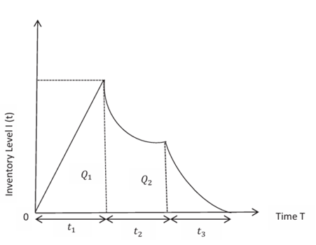
Model Formulation
The production and supply start instantaneously, and the
production ends at a time with the inventory level ![]() reached.
We assume there is no deterioration during the production uptime. In the
interval
reached.
We assume there is no deterioration during the production uptime. In the
interval ![]() ,
inventory level declines due to demand and deterioration. At the time
,
inventory level declines due to demand and deterioration. At the time ![]() ,
a markdown is offered to grow the demand rate. The position of the inventory at
any time over a period
,
a markdown is offered to grow the demand rate. The position of the inventory at
any time over a period ![]() is
governed by the following differential equation:
is
governed by the following differential equation:
|
Figure 1 |
|
Figure 1 Graphical
Representation of the System |
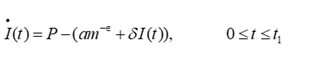 (1)
(1)
With γ=1(no
markdown) and initial boundary condition ![]() ,
,
![]() (2)
(2)
With γ=1(no
markdown) and boundary condition ![]() ,
,
![]() (3)
(3)
With boundary
condition ![]() .
.
Solution of the
above differential equations are given by:
![]() (4)
(4)
![]() (5)
(5)
![]() (6)
(6)
Where, using the
boundary condition and continuity condition, the inventory level
![]() (7)
(7)
![]() (8)
(8)
Ordering Cost = O/T
Production Cost = ![]()
Holding cost
= ![]()
Deterioration cost
= ![]()
Sales Revenue cost
= ![]()
Annual profit =
Sales revenue cost – Holding cost– Ordering cost – Production cost–
Deterioration cost
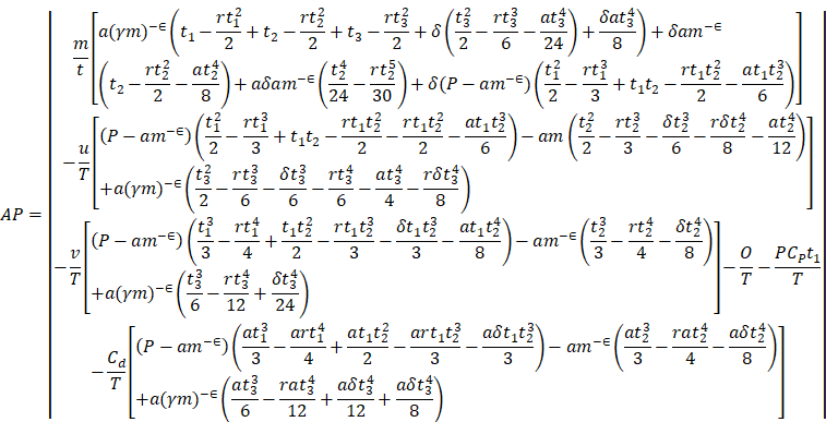
Note that Annual
Profit is a function of t1, t2 and t3. We optimize the AP function by following
Srivastava and Gupta (2013) procedure where
we rewrite,
![]()
Srivastava and
Gupta (2013) only varies T in order to find their optimal solution. However, in
our case we are able to find a better solution by varying T and ![]() . Substitute t1, t2 and t3 into equation (9),
then we obtain new equation w.r.t T and
. Substitute t1, t2 and t3 into equation (9),
then we obtain new equation w.r.t T and ![]() .
.
Solution Procedure
This sector
determines the optimum values of T and λ which maximize the total profit
AP(T, λ). The necessary condition for maximizing the AP are:
![]()
Also satisfied
with the following conditions:
![]()
Numerical
Example: In this section, a
numerical example is deliberately given to illustrate the model. The following
criteria are given below, which are used in the examples.
![]()
With these values,
the solutions of the system were found as follows:
![]()
|
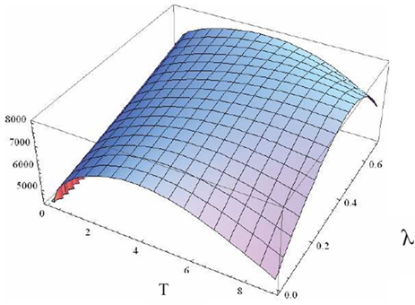
Figure 2
|
|
Figure 1 Total Cost Versus the T and |
SENSITIVITY ANALYSIS”
In order to
achieve more awareness on the issue of cost, all the parameters of +30 percent
to -30 percent are run in a sensitivity analysis. Table 1 shows the result.
Based on the sensitivity analysis, it is possible to conclude the following
insights:
|
Table 1 |
|
Table 1 Effect of
Parameters |
||||||
|
Parameters |
Change
% |
T |
λ |
Q1 |
Q2 |
AP |
|
V |
30% |
5.996 |
0.5503 |
98.973 |
661.3 |
8000.4 |
|
20% |
6.272 |
0.5314 |
103.53 |
752.97 |
8012.3 |
|
|
10% |
6.571 |
0.5122 |
108.46 |
859.7 |
8029.8 |
|
|
-10% |
7.35 |
0.4684 |
121.32 |
1171.8 |
8090 |
|
|
-20% |
7.96 |
0.439 |
131.39 |
1452.2 |
8142.5 |
|
|
-30% |
9.251 |
0.3938 |
152.7 |
2144 |
8231.7 |
|
|
30% |
7.907 |
0.4318 |
130.51 |
1737.3 |
9403.1 |
|
|
20% |
7.687 |
0.445 |
126.88 |
1511.6 |
8941.1 |
|
|
7.379 |
0.4634 |
121.8 |
1267 |
8489.6 |
||
|
-10% |
6.041 |
0.5503 |
99.71 |
635.74 |
7649 |
|
|
-20% |
0.0022 |
3896.2 |
0.0363 |
1520.8 |
3.98489×10⁷ |
|
|
-30% |
0.00056 |
-14710 |
0.00924 |
1063.4 |
1.4025×10⁸ |
|
|
δ |
30% |
6.918 |
0.4916 |
114.19 |
992.84 |
7934.6 |
|
20% |
6.918 |
0.4916 |
114.19 |
992.84 |
7974.6 |
|
|
10% |
6.918 |
0.4916 |
114.19 |
992.84 |
8014.6 |
|
|
0% |
6.918 |
0.4916 |
114.19 |
992.84 |
8094.6 |
|
|
-10% |
6.918 |
0.4916 |
114.19 |
992.84 |
8134.6 |
|
|
-20% |
6.918 |
0.4916 |
114.19 |
992.84 |
8174.6 |
|
|
-30% |
6.912 |
0.492 |
114.09 |
990.28 |
8054.2 |
|
|
Cₚ |
30% |
6.914 |
0.4918 |
114.12 |
991.33 |
8054.3 |
|
20% |
6.916 |
0.4917 |
114.16 |
992.09 |
8054.5 |
|
|
10% |
6.92 |
0.4915 |
114.22 |
993.59 |
8054.8 |
|
|
0% |
6.921 |
0.4915 |
114.24 |
993.82 |
8054.9 |
|
|
-10% |
6.924 |
0.4913 |
114.29 |
995.1 |
8055.1 |
|
|
Cd |
30% |
6.892 |
0.4903 |
113.76 |
990.96 |
8048.5 |
|
20% |
6.9 |
0.4907 |
113.76 |
991.54 |
8050.5 |
|
|
10% |
6.909 |
0.4912 |
114.04 |
992.04 |
8052.6 |
|
|
0% |
6.927 |
0.4921 |
114.34 |
993.33 |
8056.7 |
|
|
-10% |
6.936 |
0.4926 |
114.49 |
993.82 |
8058.8 |
|
|
-20% |
6.945 |
0.493 |
114.49 |
994.61 |
8060.9 |
|
|
α |
30% |
7.224 |
0.4355 |
119.24 |
1254.5 |
7842.4 |
|
20% |
7.007 |
0.4583 |
119.24 |
1119.2 |
7906.4 |
|
|
10% |
6.929 |
0.4761 |
114.3 |
1043.2 |
7977.6 |
|
|
0% |
6.95 |
0.5058 |
114.72 |
956.7 |
8137.4 |
|
|
-10% |
7.013 |
0.519 |
115.76 |
930.31 |
8226.1 |
|
|
-20% |
7.103 |
0.531 |
117.24 |
910.32 |
8321.2 |
|
|
R |
30% |
7.224 |
0.4355 |
119.24 |
1254.5 |
7842.4 |
|
20% |
7.007 |
0.4583 |
119.24 |
1119.2 |
7906.4 |
|
|
10% |
6.929 |
0.4761 |
114.3 |
1043.2 |
7977.6 |
|
|
-10% |
6.95 |
0.5058 |
114.72 |
956.7 |
8137.4 |
|
|
-20% |
7.013 |
0.519 |
115.76 |
930.31 |
8226.1 |
|
|
-30% |
7.103 |
0.531 |
117.24 |
910.32 |
8321.2 |
|
OBSERVATIONS
·
In Table
1 it is resolute on the hypothesis that it is the decrease in the parameter of
the cost of holding vcan, which in truth seeks to reduce the total cost of the
organism. The greater the increase of the v fades with increase of the cycle
time T and the larger the inventory levels Q1,Qincrease with increase of the
cycle time T, thus, the less the v, the less the markdown percentage 8.
·
As shown
in Table 1, increasing the parameter 80 of the markdown percentage +30 to
markdown percentage -10 decreases the cycle time T, annual profit, and negative
changes in the inventory level Q 1,Q 2 and negative variation in the inventory
level 1Q 2Q level with a negative change in the markdown percentage.
Nevertheless, 0.20 -20% and -30% is the unclear answer.
·
As a
fact is known, parameter C pdecreasing can lead towards the working well to
decrease the annual income of the system in table 1. It is necessary to mention
that there are no changes in other parameters because of C-pdecreases.
·
It is
clear that the reduction of the cost deterioration Cdwould bring T,Q 1,Q 2 and
maximal annual profit of the system, as shown in table 1. But it does decline
by a small percentage in the percent of markdown 4by the fall of Cd.
·
As shown
in Table 1, all the parameters are on the rise as the value of alpha decreases.
The rdecreases, but in table 1, optimum annual profit is also better and the
markdown percentage of the system λ gets better. Also, cycle time Tand
extent of stock Q decreases or increases marginally. In this regard, the lower
the quality of inventory Q2, the lower Q2 of inventory.
CONCLUSION
This paper
presents a lifetime deteriorating inventory model that has a multi-variable
demand rate. When the inventory and profit want to be maximum, then reduction
policy would be used. As this paper shows, the monetary expansion in the
business world is a good thing because it is evident in the sensitivity
analysis where effect of monetary expansion is directly pointed to be the
optimal markdown time and optimal cost. Cost is taken to be a variable function
because to bring the study closer to reality which increases as time
progresses. It is also possible to determine that policy makers must be very
keen to make the reduction rate dependent. The proposed model can be
generalized in cases of partial backorder, stochastic demand and the other one
is permitable delay in payment.
ACKNOWLEDGMENTS
None.
REFERENCES
Ghare, P. M., and Schrader, G. F. (1963). An Inventory Model for Exponentially Deteriorating Items. Journal of Industrial Engineering, 14, 238–243.
Goyal, S. K., and Giri, B. C. (2001). Recent Trends in Modeling of Deteriorating Inventory. European Journal of Operational Research, 134(1), 1–16. https://doi.org/10.1016/S0377-2217%2800%2900248-4
Jaggi, C. K. (2014). An Optimal Replenishment Policy for Non-Instantaneous Deteriorating Items with Price Dependent Demand and Time-Varying Holding Cost. International Scientific Journal on Science, Engineering and Technology, 17(3).
Nagare, M., and Dutta, P. (2018). Single-Period Ordering and Pricing Policies with Markdown, Multivariate Demand and Customer Price Sensitivity. Computers and Industrial Engineering, 125, 451–466. https://doi.org/10.1016/j.cie.2018.09.004
Omar, M., and Zulkipli, H. (2014). An Integrated Just-in-Time Inventory System with Stock-Dependent Demand. Bulletin of the Malaysian Mathematical Sciences Society, 37(4).
Singhal, S., and Singh, S. R. (2017). Supply Chain System for Time and Quality Dependent Decaying Items with Multiple Market Demand and Volume Flexibility. International Journal of Operational Research, 31(2). https://doi.org/10.1504/IJOR.2018.089131
Singh, S. R., and Sharma, S. (2018). A Partially Backlogged Supply Chain Model for Deteriorating Items Under Reverse Logistics, Imperfect Production/Remanufacturing and Inflation. International Journal of Logistics Systems and Management, 33(2). https://doi.org/10.1504/IJLSM.2019.100113
Singh, S. R., and Rana, K. (2020). Effect of Inflation and Variable Holding Cost on Life Time Inventory Model with Multi-Variable Demand and Lost Sales. International Journal of Recent Technology and Engineering, 8(5). https://doi.org/10.35940/ijrte.E6249.018520
Singh, S. R., and Rana, K. (2020). Optimal Refill Policy for New Product and Take Back Quantity of Used Product with Deteriorating Items Under Inflation and Lead Time. In Strategic System Assurance and Business Analytics. https://doi.org/10.1007/978-981-15-3647-2
Tayal, S., Singh, S. R., Sharma, R., and Singh, A. P. (2015). An EPQ Model for Non-Instantaneous Deteriorating Item with Time Dependent Holding Cost and Exponential Demand Rate. International Journal of Operational Research, 23(2), 145–161. https://doi.org/10.1504/IJOR.2015.069177
Widyadana, G. A., and Wee, H. M. (2007). A Replenishment Policy for Item with Price Dependent Demand and Deteriorating Under Markdown Policy. Jurnal Teknik Industri, 9(2), 75–84. https://doi.org/10.9744/jti.9.2.75-84
Wang, X., Fan, Z. P., and Liu, Z. (2016). Optimal Markdown Policy of Perishable Food Under the Consumer Price Fairness Perception. International Journal of Production Research, 54(19), 5811–5828. https://doi.org/10.1080/00207543.2016.1179810
 This work is licensed under a: Creative Commons Attribution 4.0 International License
© Granthaalayah 2014-2026. All Rights Reserved.