INVERSE EXPONENTIATED EXPONENTIAL POISSON DISTRIBUTION WITH THEORY AND APPLICATIONS

 

Lal Babu Sah Telee ¹, Vijay Kumar ² 

 

¹ Assistant Professor, Department of Management Science, Nepal Commerce Campus, Tribhuvan University, Kathmandu, Nepal

²  Professor, Department of Mathematics and Statistics, Deen Dayal Upadhyaya, Gorakhpur University, Gorakhpur, India

 

1. INTRODUCTION

Statistical distributions are the basic aspects of all parametric statistical techniques including inference, survival analysis, modelling and reliability etc. In recent years, new generate families of continuous models are derived. Lifetime problems can be solved by using the existing probability models but to get more precise result, we need some flexible probability models. Due to constant failure rate, exponential model cannot explain data with variable failure rate. Hence, misuse of exponential lifetime model will not be suitable. Here, our aim is to introduce a new three parameter lifetime distribution with strong physical motivations. At present many of new models are proposed by modifying, merging, and adding or removing some parameters in existing models Marshall and Olkin (2007). That is existing models can be defined in new family of distributions. Several techniques can be defined to form new family of distribution adding some extra parameters to the existing distributions Rinne (2009). and Pham and Lai (2007).

CDF of the continuous random variable X following exponential distribution having constant   is given as,

 

                          .

 

Some alternative generalizations of exponential distribution have been proposed to give some flexibility.

Although there are several generalizations of the exponential distributions, following two distributions have received more attention in literature with respect to others.

·        Marshall & Olkin (1997) introduced inventive general method by adding some parameters to family of distributions which states that X have the Marshall-Olkin extended exponential (MOEE) distribution, say  as

 

                           

 

Here  are called tilt and scale constants. MOEE model reduces to exponential distribution for  equal to 1.

·        Generalize: exponential (GE) distribution Gupta and Kundu (1999) can have decreasing and right skewed with single mode value. Let X follows GE distribution. That is. The CDF of X is given by

 

                           

 

Above distribution has expression of the survival function like Weibull distribution and properties similar to Gamma distribution.

To derive this model, we have used exponential distribution and the Poisson distribution. Let us consider N system-based plant working independently where N is truncated Poisson rv. Suppose each of the system contains independent and identically distributed units arranged in parallel. Suppose X is a random variable defining time to fail the system Ristić & Nadarajah (2014) and Kus (2007) then probability mass function of the N will be.

 

                           

 

where n = 1, 2, 3…

Unconditional CDF of X having three parameters was introduced and was named as EEP Ristić & Nadarajah (2014) distribution

 

                

 

We have defined here three parameters Inverse Exponentiated Exponential Poisson distribution (IEEP) taking inverse of random variable X with CDF

 

            

 

2. Model Analysis

2.1. Inverse Exponentiated exponential Poisson (IEEP) Distribution

Let X follows new extended exponential distribution then CDF of the proposed model having three parameters is,         

 

                               (1)

 

2.2. Probability Density function

We defined model with pdf in expression as

 

                                  (2)

 

2.3. The Reliability function

It is defined as probability of not failing an event before given time t. Reliability function of IEEP is

 

 ; x > 0                                        (3)

 

2.4. The hazard rate (HRF)

Hazard function rate is defined as the instantaneous failure rate at time t. HRF of proposed model is

 

 

 

; x > 0                      (4)

 

Some of density function curves and hazard curves of IEEP using some of values of and  are plotted in Figure 1 at constant value of λ = 2 indicating that density curve of the IEEP is of different shapes at different parameters values.

Figure 1

                                                                             

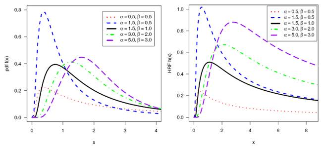
Figure 1 The PDF (Left) and HRF(Right) of IEEP for Various Values of   and   Taking λ = 2

 

Behaviour of the hazard rate shows high flexibility for different values of parameters. The HRF curve shows that the function is unimodal. Function is monotonically increasing along with monotonically decreasing. It is inverted bathtub hazard rates not showing constant hazard rates.  We know that many of the lifetime’s distribution does not show upside-down bathtub hazard rates, but it exhibits in case of proposed model.

 

2.5. Statistical Properties

Major characteristics such as quantile function, skewness, and kurtosis etc of the proposed model IEEP are derived in this section.

 

2.6. Quantile Function

To study the theoretical aspect of probability model, quantile function is used. Statistical measures like, partition values, skewness as well as kurtosis of the probability models can be studied using quantile function. Generating function of random variable can be expressed in terms of quantile function. Quantile function can be used as the alternative function of PDF and CDF for finding the nature of the distributions. Quantile function of function can be obtained by using the relation Quantile function for model IEEP is,

 

 

 

  ; 0 < u < 1.                                  (5)

 

U is uniform variate U (0, 1). If we put u = 0.5 in (5) then median will be obtained of the model can be obtained.

 

2.7. Asymptotic properties

This property of pdf the density function follows condition of   with the resulting value as 0. That is, if both the limits converge to zero the proposed model satisfies the asymptotic behavior indicating that model value exists.

 

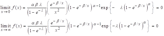              (6)

 

Since both the limits exist and have the limiting values as zero, we confirm that the proposed modal has unique mode. The necessary and sufficient conditions for mode are and  By using these necessary and sufficient conditions, mode of the proposed model is obtained as,

 

                    (7)

 

2.8. Skewness and Kurtosis

These are the measures that describe the nature like consistency of data and the normality of probability distribution. Bowley's skewness Al-Saiary et al. (2019) based on quartiles can be calculated using expression as

 

                    

 

Moors (1988) and Al-Saiary et al. (2019) introduced kurtosis using Octiles given by the relation.

 

                   

 

 Q (.) is quantile functions of the model.

Statistical measures of this new model are obtained. For this, 100 random samples from the quantile function mentioned in expression (5). Here, we have taken initial values of the parameters as. By using the generated values different basic statistics of the proposed model are calculated. Table 1 Mean, Median, Mode, Sd, Skewness and Kurtosis of IEEP contains summaries for some set of parameters.

Table 1

Table 1 Mean, Median, Mode, Sd, Skewness and Kurtosis of IEEP
α	β	λ	Mean	Median	Mode	Sd	Skewness	Kurtosis
40	20	2	6.75	6.57	6.21	1.416	0.535	3.245
39.5	20	2	6.67	6.6	6.64	1.416	0.54	3.25
38.5	22	2	6.83	6.643	6.27	1.448	0.546	3.26
41	22	2	6.701	6.525	6.173	1.396	0.527	3.236
42	22	2	6.653	6.481	6.137	1.376	0.52	3.227
40.5	21.5	2	6.726	6.548	6.192	1.406	0.531	3.24
40	20	2	6.751	6.571	6.211	1.416	0.535	3.245
40	23	2.5	6.95	6.775	6.425	1.397	0.526	3.275
40	23	3	7.133	6.959	6.611	1.375	0.53	3.31

 

Standard deviation is decreasing when values of are increasing. Also values of  are decreasing. Values of skewness as well kurtosis is not unique showing that distribution is skewed and not normal in nature.

 

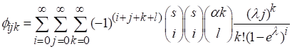
2.9. Some Expansions

Following distribution is derived for studying the various characteristic of the model by application of generalized binomial series. Taking  we can write.

                 

 

The power series expansion of corresponding to an exponential function is;

 

                            

 

Using above two binomial series and exponential expansion in given pdf equation, the proposed model in series form is.

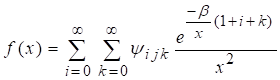                                                                          (8)

 

Where,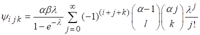  

 

3. Calculation of moments

Quantitative measurements of the distribution in form of function that describes characteristics of the probability distributions can be explained using moments. The  raw moment  new modelis given as

                                                                                   (9)

 

Integrating equation (9), we can get  raw moments of the IEEP can be obtained as

                            

 

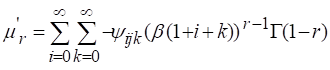
When r =1 then mean of the IEEP will be as

                              

 

Second order raw moment of IEEP can be obtained taking r as 2. That is.

                             

 

Using relation,, variance can be obtained. Mean median and others measures of the proposed model are given above in Table 1 Mean, Median, Mode, Sd, Skewness and Kurtosis of IEEP. Lower incomplete moments  is given by

                                                                                              (10)

 

Lower incomplete gamma function and density functions are used to 

find lower incomplete moment as

 

                             

 

The conditional moments is

                                                                                               (11)

 

Upper incomplete gamma function is

 

                             

 

Using density function and upper incomplete gamma function in equation (11), we can get conditional moment as.

 

                            

 

Similarly, MGF of the proposed model is given as;

 

                             

 

Hence, we can get MGF as

 

                                                         (12)

 

3.1. Residual Life Function

Here,moment of the residual life of random variable X of the IEEP can be defined by

                            

 

Expression  can expanded using binomial series expansions as,

 

                              

 

Hence,  moment of residual life of X of the distribution becomes.

 

 

                               (13)

 

Using upper incomplete gamma function in (13), we have

 

                                                                                

 

Also,   moment of revised residual life function of X of the proposed model IEEP is found as

                           

 

Applying binomial expansion and substituting pdf, we can get following expression.

                                                                               

 

3.2. The probability Weighted Moment

The probability weighted moment can be obtained using relation

 

                                                          (14)

 

Applying the expansion of

 

                                                                                                    (15)

Where,

 

 

Now, using equations (14) and (15), we can write

 

                                                       (16)

 

Integrating equation (17), we get

 

                                                                                 

 

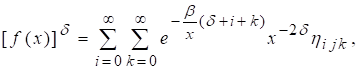
3.3. Order Statistics

 Let  is order statistics of any sample of size n from IEEP. The PDF of order statistics David & Nagaraja (2004) is defined as,

 

                                   (17)

 

Where  denotes the beta function. Substituting the values of PDF and equation (16) replacing s by, we get

 

                   (18)

 

Where,       

 

Now moment of the order statistics is

 

                                                                         (19)

 

Using equations (18) and (19) the  moment of the order statistics become

 

3.4. R'enyi and q-entropies

The entropy is used in many fields such as in statistics, mathematics, engineering, physics, thermodynamics etc. It can be used to measures the variation of uncertainty of the random variable R'enyi entropy is defined as;

 

                                 (20)

 

Applying the expansion of

                                               (21)                    

               

                                                                              where,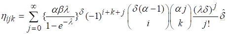     

 

From equation (20), we can write

 

       

 

Similarly, we can define q-entropy as;

 

                                                                                        

 

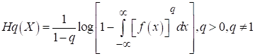
Thus, we can define the q-entropy is as.

 

          

 

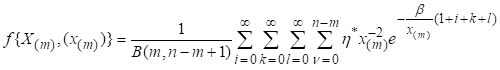
4. Parameter Estimation Technique

4.1. Estimation using Maximum Likelihood

Here we found the MLE of the parameters for constructed model. The MLE of the parameters are based on the observed sample x₁, x₂,…,x_n. The likelihood function of parameters  is given by

 

                  (22)

 

Log likelihood function  is given by

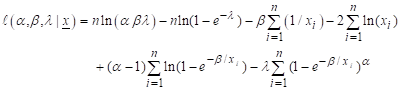                                  (23)

 

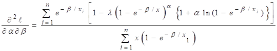
Here, differentiating the log likelihood function (23) and maximum likelihood estimators were obtained by equating the differentiated equations to zero. That is

 

                     (24)

 

                                 (25)

 

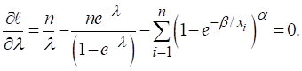                                                    (26)

 

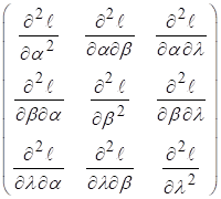
Estimation of unknown parameters is done by solving nonlinear equations (24), (25) and (26). It will be difficult in solving these equations analytically so Newton- Rapson's iteration techniques is applied in log likelihood function of equation (23) using function of R. Let  is MLE of  Asymptotic normality result is. The fisher's information matrix  given by;

 

=              

 

The maximum likelihood estimates (MLE)  of was obtained by solving three nonlinear equations analytically and using statistical software.

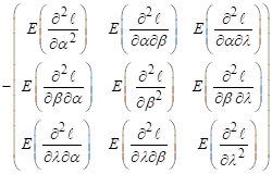
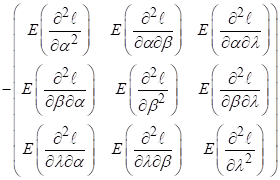
The  CI for constants  and  are obtained. Here we have used asymptotic normality of MLE method and Variances of estimated parameters using the inverse of of second derivatives of log likelihood function. The second order derivatives are

 

           

 

 

 

 

 

 

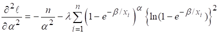
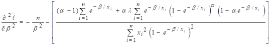
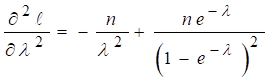
Let is the parameter vector and  be corresponding MLE. This provides (- )  N (0, ( ) ) as asymptotic normal where is fishers information matrix given by

  = 

 

It will be worthless that MLE gives asymptotic variance.  Approximation of the asymptotic variance can be done by taking estimated values of the parameters. For this fisher’s information matrix    which is given as;

  = -  =    where H is the hessian.

 

We can obtain the observed information matrix maximizing the likelihood. For this Newton Rapshon algorithm is used. We have also find expression of variance covariance matrix as

=

 

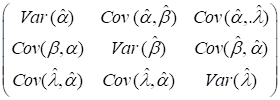
Hence from asymptotic normality of MLE approximate   100(1- ) % CI for the parameters are constructed using upper percentile standard normal variate as, 

 

 

 

where  is the upper percentile of standard normal variate.

 

5. Applicability and data analysis

5.1. Data set

This section represents analysis of real dataset to verify the proposed model. Sometimes electro migration can occur in circuit because failures in microcircuit happen due to the movement of atoms in the circuits. Data is from an accelerated life test that includes 59 conductors Schafft et al. (1987); Nelson and Doganaksoy (1995) where failure time is measured in hours with no any censoring of the observations.

4.700, 6.545, 9.289, 7.543, 6.956, 6.492, 5.459, 8.120, 4.706, 8.687, 2.997, 8.591,6.129, 11.038, 5.381, 6.958, 4.288, 6.522, 4.137, 7.459, 7.495, 6.573, 6.538,5.589, 5.807, 6.725, 8.532, 9.663, 6.369, 7.024, 8.336, 9.218, 7.945,6.869, 6.352, 6.087, 6.948, 9.254, 5.009, 7.489, 7.398, 6.033, 10.092, 7.496, 7.974, 8.799, 7.683, 7.224, 7.365, 6.923, 5.640, 5.434, 7.937, 6.515, 6.476, 6.071, 10.491, 5.923 ,4.531.

 

5.2. Descriptive Data Analysis

Exploratory data analysis is a collection of different statistical analysis that explains and to summarize the data set used in research. Objective of this is to gain detailed idea of data set used. It may include some descriptive statistics as well as the graphical plots of the data. Following are main measures that can be included in descriptive data analysis.

·        The boxplot, histogram, density curve etc. These are a graphical plot that help to find the pattern of the data and also helps to detect if there is any unusual pattern and observations in data.

·        Measures of location, measures of scatters, skewness, and kurtosis etc gives some specific aspect and nature of the data.

R programming language is used to find summary of the data and the values obtained are tabulated below in table

Table 2

Table 2 Descriptive Statistics
Min.	Q1	Q2	Mean	Q3	Max.	Skewness	Kurtosis
2.997	6.052	6.923	6.98	7.941	11.038	0.193	3.088

 

Figure 2 represents the boxplot and the histogram & and density fit of the proposed model IEEP.

Figure 2

                                                                      

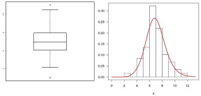
Figure 2 Boxplot (Left Panel) and Histogram and Fitted Density Plot (Right Panel)

 

6. Parameter estimation                                  

There are various methods and tools for optimization of the function. Forgetting maximum likelihood estimates (MLE) of the defined model log-likelihood function defined in expression (23) is maximized. The maximum likelihood estimates their standard error along with 95% confidence Interval (CI) for parameters  and is obtained using R programming [R Development core Team, (2016)]. We have also used the quasi-Newton-Raphson algorithm in R [Rizzo, 2008] for maximum likelihood estimation.

Table 3

Table 3  MLE, Standard Error and 95 Percent C. I
Parameters	MLEs	Standard Error	95% C.l.
alpha	40.5868	4.86	(31.068, 50.113)
beta	22.7553	2.049	(18.739, 26.771)
lambda	2.9968	1.251	(0.5450, 5.4490)

 

The profile plots of negative log-likelihood function of proposed model for   and are plotted separately and are shown in Figure 3.

Figure 3

                                                                      

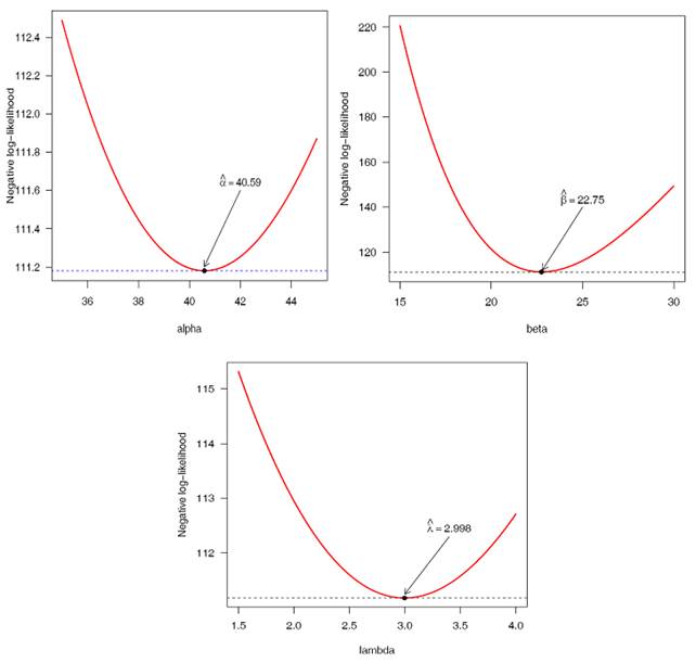
Figure 3 The Profile of Negative Log-Likelihood Functions of  and

 

Parameters and standard errors of IEEP and other models such as Exponentiated Exponential Poisson (EEP) Joshi (2017) Distribution, Logistic Inverse Exponential (LIE) Chaudhary and Kumar (2020), The Kumaraswamy Half-Cauchy distribution (KSHC) Ghosh (2014) distribution are estimated and are compared for the comparisons of the proposed model. Estimated parameters using MLE are mentioned in Table 4.

Table 4

Table 4 MLE and Standard Error of IEEP and the Other Distributions
Probability model
IEEP	40.5868(31.0160)	22.7553(2.0490)	2.9968(1.2510)
EEP	9.8700(4.5008)	0.1774(0.0995)	21.0934(27.1612)
LIE	5.3220(0.5830)	-	4.7357(0.1433)
KSHC	8.8568(5.7731)	118.5980(119.7700)	5.7472(4.9376)

 

 

6.1. Model Comparison

Here, log-likelihood as well as the information criteria values like  (i) Akaike's information criteria (AIC), (ii) Bayesian information criteria(BIC) (iii) Corrected Akaike's information criteria(CAIC), and (iv) Hannan-Quinn Information Criteria(HQIC)are calculated and tabulated in Table 2 and Table 5 Following relations are used to find the values of AIC, BIC, CAIC and HQIC.

 

    ,;      

 

       and   

 

   .

 

where n and k are total number of samples and total number of constants respectively. Since IEEP has least information criteria values with respect to the other competing, it is considered that IEEP fits data well.

Table 5

Table 5 AIC, BIC, CAIC and HQIC of IEEP and Other Models
Probability model	AIC	BIC	CAIC	HQIC
IEEP	228.35	234.59	252.35	231.523
EEP	228.65	234.88	252.65	231.813
LIE	232.053	238.286	244.053	232.16
KSHC	880.37	886.61	904.377	883.541

 

7. Model validation

For model validation, we can use different statistical techniques. Here we have used two types of graphical plots; probability versus probability (P-P) plots and quantile versus quantile (Q-Q) plots are drawn and are shown in Figure 5. PP and QQ plots show the theoretical distribution versus distribution. A P-P plot describes the points;  =              and  is order statistics of proposed model. , is termed as the empirical distribution function, and  is the indicator function.  In same way, the QQ plot depicts the points;

 

                               .

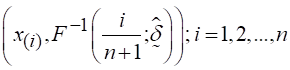Figure 4

                                                                      

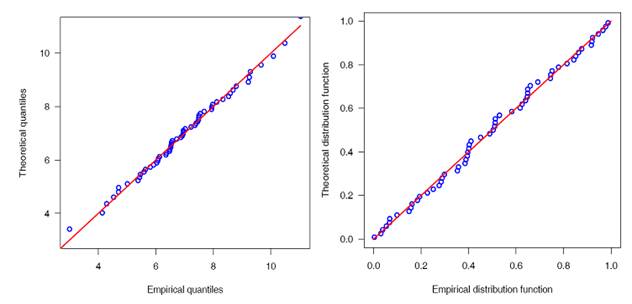
Figure 4 P-P Plot in Left Panel and Q-Q Plot in Right Panel of the IEEP

 

The IEEP fits better in both the empirical and fitted case of distribution function. For model validation, Kolmogrov - Smirnov test showed D = 0.0520 with p-value = 0.9947 which means the model fits significantly. Curve for empirical distribution function and the fitted distribution function are plotted and is displayed in Figure 6

Total Time Test (TTT) plot is also shown in right panel of the Figure 6. The Empirical version of TTT plot is given as

             

 

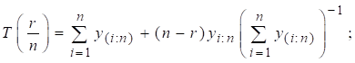
Where, r = 1, 2... n and  be sample order statistics. Concave shape of Curve of the TTT plot shows that hazard rate curve is increasing.

Figure 5

                                                                       

Figure 5 Theoretical Versus Empirical Plot (Left) and TTT Plot (Right)

 

Figure 6 in left panel displays the empirical distribution curve and the fitted distribution curve for the newly defined model corresponding to other models. In Right panel of the Figure 6, histogram of the data and fitted density curve of the model under study and the competing models are displayed.

Figure 6

                                                                      

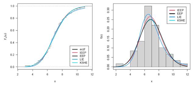
Figure 6 Estimated Fitted CDF with EDF (Left) and Estimated Fitted PDF

 

8. Summary and Conclusion

This article is based on derivation, study and application of newly introduced probability model having three parameters. It is name as Inverse Exponentiated Exponential Poisson Inverse along with some statistical and mathematical properties, probability, weighted moments, order statistics, skewness, kurtosis, residual life time, entropy and survival functions etc. Different information criteria values are obtained for both the IEEP and the considering model and are compared. Study also showed that the goodness of fit statistics has least test statistics and higher p value respective to the other considering model. We have also plotted the empirical cdf versus the fitted cdf as well as the histogram versus the fitted density plot of the models. All the statistical computations and the graphical measures are performed using R language programming.

 

CONFLICT OF INTERESTS

None. 

 

ACKNOWLEDGMENTS

None.

 

REFERENCES

Al-Saiary, Z. A., Bakoban, R. A., & Al-Zahrani, A. A. (2019). Characterizations of the Beta Kumaraswamy Exponential Distribution. Mathematics, 8(1), 23. https://doi.org/10.3390/math8010023.

Chaudhary, A. K., & Kumar, V. (2020). Half Logistic Exponential Extension Distribution with Properties and Applications. International Journal of Recent Technology and Engineering (IJRTE), 8(3), 506-512. https://doi.org/10.35940/ijrte.C4625.099320.

David, H. A., & Nagaraja, H. N. (2004). Order Statistics. John Wiley & Sons. https://doi.org/10.1002/0471667196.ess6023.

Ghosh, I. (2014). The Kumaraswamy-Half-Cauchy Distribution : Properties and Applications. J. Stat. Theory Appl., 13(2), 122-134.  https://doi.org/10.2991/jsta.2014.13.2.3.

Gupta, R. D., & Kundu, D. (1999). Theory & Methods : Generalized Exponential Distributions. Australian & New Zealand Journal of Statistics, 41(2), 173-188. https://doi.org/10.1111/1467-842X.00072.

Joshi, R. K. (2017). The Analysis of Some Statistical Models. Doctoral Dissertation in Statistics Submitted to Deen Dayal Upadhyaya Gorakhpur University, Gorakhpur. 

Kus, C. (2007). A New Lifetime Distribution. Computational Statistics & Data Analysis, 51, 4497-4509. https://doi.org/10.1016/j.csda.2006.07.017.

Marshall, A.W., & Olkin, I. (1997, September). A New Method for Adding a Parameter to a Family of Distributions with Application to The Exponential and Weibull Families. Biometrika, 84(3), 641-652. https://doi.org/10.1093/biomet/84.3.641.

Marshall, A. W., & Olkin, I. (2007). Life Distributions, 13.

Moors, J. (1988). A Quantile Alternative for Kurtosis. The Statistician, 37, 25-32. https://doi.org/10.2307/2348376.

Nelson, W., & Doganaksoy, N. (1995). Statistical Analysis of Life or Strength Data from Specimens of Various Sizes Using the Power-(Log) Normal Model. Recent Advances in Life-Testing and Reliability, 377-408. https://doi.org/10.1201/9781003418313-21.

Pham, H., & Lai, C. D. (2007). On Recent Generalizations of the Weibull Distribution. IEEE Transactions on Reliability, 56(3), 454-458. https://doi.org/10.1109/TR.2007.903352.

Rinne, H. (2009). The Weibull Distribution : A Handbook. CRC Press, Boca Raton. https://doi.org/10.1201/9781420087444.

Ristić, M. M., & Balakrishnan, N. (2012). The gamma-exponentiated exponential distribution. Journal of statistical computation and simulation, 82(8), 1191-1206. https://doi.org/10.1080/00949655.2011.574633.

Ristić, M. M., & Nadarajah, S. (2014). A new lifetime distribution. Journal of Statistical Computation and Simulation, 84(1), 135-150. https://doi.org/10.1080/00949655.2012.697163.

Schafft, H. A., Station, T. C., Mandel, J., & Shott, J. D. (1987 Feb 24). Reproducibility of Electro-Migration Measurements, IEEE Transactions on Electron Devices, ED-34, 673-681. https://doi.org/10.1109/T-ED.1987.22979.