Developing a multi-objective sustainable supply chain network location-allocation model for perishable products

 

Shadi Munshi ¹, Abdul Aziz Al-Anazi ¹, M. S. Al-Ashhab ^{1, 2}

 

¹ Department of Mechanical Engineering, College of Engineering and Islamic Architecture, Umm Al-Qura University, Makkah 24211, Saudi Arabia

² Design and Production Engineering Department Faculty of Engineering, Ain-Shams University, Cairo 11511, Egypt

 

 

1. INTRODUCTION

Some researchers defined Supply chain management (SCM) as the automatic integration of stakeholders starting with demand from customers and passing by needs from suppliers according to the estimation of the enterprise resource planning system Al-Ashhab et al. (2021). The term "supply management" may be considered for the management of systems to optimize costs of materials, quality, and service Dai et al. (2018). To achieve this optimization, the following operations should be integrated: procurement, transportation, storage, required quality assurance to manage the inventory of materials, as well as the internal distribution of resources. Material Management in the organization includes all aforementioned activities Isaloo and Paydar (2020)

During manufacturing planning activities, the design of SCN plays a vital role in any firm. So, the decision of SCN design is one of the most important taken one in SCN. the design is considered strategic planning of the supply chain Rashidi et al. (2016) It plays a major role in SCM.

Exact methods have been used to solve SSCN design including heuristics plus metaheuristics, LP, NLP, and MILP. Moreover, MINLP models have been also developed (MINLP) Al-Ashhab and Aldosari (2022). GAMS platform could be used for implementing this mathematical formulation Al-Ashhab and Aldosari (2022), GAMS (n.d.). Metaheuristic algorithms are also used based on Pareto solutions Rashidi et al. (2016), Zahiri et al. (2017), as in the Genetic Algorithm (GA) Dai et al. (2018), Rashidi et al. (2016), Rohmer et al. (2019), Validi et al. (2014) Gas, as a population-based technique works effectively for multi-objective optimization problems. Konak et al. (2006) Holland et al developed the concept of GA in the early 1960s and 1970s (Rate & a Cue, n.d.).

Schaffer (1985) has proposed the first multi-objective GA, called vector evaluated GA (or VEGA). Niched Pareto Genetic Algorithm (NPGA), Subsequently, Horn et al. (1994) developed several multi-objective evolutionary algorithms, including the multi-objective Genetic Algorithm (MOGA) Kocabay and Alaçam (2017) the Weight Based Genetic Algorithm (WBGA) Hajela and Lin (1992) Random Weighted Genetic Algorithm (RWGA) Konak et al. (2006) Non-dominated Sorting Genetic Algorithm (NSGA) (Konak et al., 2006). Particle Swarm Optimization (PSO) Patidar et al. (2018), and Simulated Annealing (SA) Chalmardi et al. (2019), Eskandari-Khanghahi et al. (2018)

ε-constraint technique, is also used by researchers Arvan et al. (2015), Rohmer et al. (2019) Some of them devised a solution strategy to solve their model, based on Lagrangian relaxation and ε-constraint Diabat et al. (2019) Some models Isaloo and Paydar (2020), Yakavenka et al. (2020) Production and distribution planning are the two main optimization problems in the supply chain and their decisions are often made separately. The process begins with production and then continues to product distribution from manufacturers to consumers. However, competition resulting from globalization, and various competitors in the local market requires that the supply chain in the company guarantee its resource efficiency, increase its service level for consumers, and reduce lead time and stock Herlina (2022)

The profit and overall service level of the customers are greatly affected by production planning effects. Therefore, it is very important to pay more attention to the production planning process to ensure a high-profit level and high service level on the other side Al-Ashhab (2016) Other aspects such as environmental or economic impact, have urged academic researchers to consider them due to their importance. Some of them created bi-objective models that took into account both economic and environmental objectives, in which environmental consequences, are designed to reduce CO2 emissions Al-Ashhab et al. (2021) as in designed proposed models. The main or first objective Trisna et al. (2016) is to minimize total cost in the framework of multi-objective function in the supply chain.

This study discusses the design and plan of an SSCN for perishable products to maximize SC profit, and the OCSLs, and minimize total cost. A mathematical model has been devised to design a multi-period model that is sustainable for three suppliers, a manufacturer, a retailer, and one warehouse. The problem is reformulated using MINLP.

The model's aim is to find out the best supply chain configuration is and how many units should be produced in each period without extraneous manufacturing efforts, as well as the number of units to be moved from the manufacturer to the warehouse and from the warehouse to the consumer. Perishability of products, retailer demand, and inventory management will be based on the ages of products in the warehouse. As for perishable goods, the FIFO inventory policy is commonly used by producers, when it is preferred in the real-world sector since it prevents product waste and expiration.

Figure 1 shows the SCN as it consists of three potential suppliers, three potential manufacturers, and one warehouse to serve three customers.

Figure 1

                                                                          

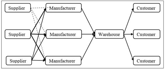
Figure 1 Supplier, Manufacturer, Warehouse, and customer network

 

2. MATHEMATICAL MODEL FORMULATION

2.1. NOTATIONS

 

Sets

S        Suppliers.

M       Manufacturers.

W      Warehouse.

C        Customers.

A        Ages of stored products.

T        Planning periods.

 

Parameters

              Shelf-life.

 The demand of customers.

        Supplier capacity.

   Manufacturer capacity.

    Hour’s capacity of manufacturer.

      Warehouse capacity.

              Price of customers.

               Fixed cost of contracting supplier.

              Fixed cost of opening manufacturing.

              Fixed cost of warehouse.

              Transportation cost per unit per distance.

            Big number.

         Distance between manufacturer and warehouse.

            Distance between supplier and manufacturer.

            Distance between warehouse and customers.

            Inventory retention cost.

              Expired cost.

               Batch size from supplier.

             Batch size from manufacturer.

             Batch size from warehouse.

   Material cost per unit supplied by supplier.

            Manufacturer capacity cost per hour of the facility that is not utilized.

               Shortage cost.

            Material cost per unit for manufacturer.

 

Variables     

The number of batches transported from supplier to the manufacturer.

 The number of batches transported from manufacturer to the warehouse.

The number of batches transported from warehouse to the customer.

      Inventory of age at the end of period.

Expired inventory at the end of period.

       Binary variable equals 1 if facility i is open and 0 otherwise.

 Binary variable equals 1 if a transportation link is activated between (w) and (m).

 Binary variable equals 1 if a transportation link is activated between (s) and (m).

 Binary variable equals 1 if a (c) is contracted and 0 otherwise.

          Total profit.

          

2.2. OBJECTIVES FUNCTIONS

The objectives of the model are to maximize the profit, OCSLs of the three customers Equation 1 and consequently minimizing the total cost.

Subtraction of the total cost Equation 3, Equation 10 from the total revenue Equation 2 will result in the total profit.

 

    Equation 1

 

                                                         Equation 2

 

Total cost = fixed costs + material costs + non-utilized capacity costs + shortage costs + transportation costs + manufacturing costs + inventory holding costs.

 

                                              Equation 3

 

                                      Equation 4

 

                               Equation 5

 

                                                                            Equation 6

 

              Equation 7

 

                                                          

                Equation 8

 

                                      Equation 9

 

                                                                 Equation 10

 

2.3. CONSTRAINTS

The following section represented constraints of the proposed model.

 

                                                                        Equation 11

 

Constraint Equation 11 ensures that the supplier’s capacity does not exceed the sum of the flow exiting from each supplier to manufacturer, at each period.

 

                                                                    Equation 12

 

Constraint Equation 12 guarantees that the manufacturer's pre-specified capacity doesn’t exceed the number of units transferred from manufacturer to supplier.

 

                                                  Equation 13

 

Constraint Equation 13 ensures that the sum of production hours for all products manufactured in the warehouse is delivered to its store, in each period that does not exceed manufacturing capacity hours.

 

                                                                               Equation 14

 

Constraint Equation 14 guarantees that the pre-selected capacity from the manufacturer will be equal to the number of units transferred from manufacturer to supplier.

 

                                                                                          Equation 15

 

Constraint Equation 15 guarantees that the warehouse capacity in the first period does not exceed the number of units transferred from the manufacturer to the warehouse.

 

                                                  Equation 16

 

Constraint Equation 16 guarantees that the total quantity of products entering the warehouse will not be exceeded the warehouse's pre-specified capacity, in each period and products remaining from the previous period.

The FIFO policy is the best for the inventory of perishable products which has a short shelf life by its nature, to prevent product expiration and minimize the costs arising from those expired products as the policy prioritizes maximizing of the use of inventory by the oldest products that will be deteriorated first.

 

                                                         Equation 17

 

Equation 18

 

                                                                                                                                 Equation 19

 

Constraints Equation 17, Equation 19 the warehouse at the end of each period is calculated by remaining inventory. They guarantee that the FIFO inventory policy has been applied. FIFO inventory policy will be used first to fulfil demand. The distribution age of the units in stock is monitored then the inventory of the intermediate age, and finally the demand will be fulfilled by inventory of the lowest age or the inventory of the freshest units.

 

                                                                               Equation 20

 

                                                                      Equation 21

 

Constraint Equation 20 guarantees that no expired inventory will arrive at the shelf-life. Moreover constraint Equation 21 calculates the expired inventory that only appears after reaching shelf life.

As a result of adopting the FIFO inventory policy, the environmental impact is minimized by preventing the expiration of the products. Producing a sufficient quantity from the manufacturer to the warehouse according to the retailers’ demands and withdrawing from the old demand (FIFO), will result in the prevention of product expiration, in case of storing some quantities for the next periods. Saving the environment by preventing the expiration of production is important, as many energies and resources can be saved in processes, i.e., material, production, transportation, etc.

 

3. COMPUTATIONAL RESULTS AND ANALYSIS

3.1. MODEL VERIFICATION

The model which comprises six planning periods, three potential manufacturers, warehouse, and three customers. All the inputs in the experiments have fixed variables as presented in Table 1. It’s assumed that retailer demand values in the six periods are 5000, 6000, 7000, 8000, 9000, and 10000 units, respectively.

Table 1

Table 1 Model parameters
Parameter	Value	Parameter	Value
	10000 ($)		100 ($)
	3 (Period)		10 ($)
	15 ($)		10 ($)
	10 ($)		30, 40, 50 (Km)
	0.002 ($)		40, 50, 30 (Km)
	4 ($)		50, 30, 40 (Km)
	3 ($)		200, 100, 400 (Km)
	1		200, 250, 300 (Km)
	1		6000 (unit)
	1		6000 (unit)
	10000		6000 (hour)
	20000		600000 (unit)

 

3.2. RESULTS AND ANALYSIS

The number of units transferred from suppliers to manufacturers, the number of units transferred from the manufacturer to the warehouse, warehouse to the customer, and the inventory and expired quantities are presented in Table 2 and Table 3, Table 4 shows that the FIFO strategy has been used successfully to avoid aging of stored products and avoid expiration at a 0% deviation.

Table 2

Table 2 Number of units transferred from suppliers to manufacturers
	Supplier 1			Supplier 2			Supplier 3
Period	S1M1	S1M2	S1M3	S2M1	S2M2	S2M3	S3M1	S3M2	S3M3
1	6000	0	0	0	6000	0	0	0	6000
2	6000	0	0	0	6000	0	0	0	6000
3	6000	0	0	0	6000	0	0	0	6000
4	6000	0	0	0	6000	0	0	0	6000
5	6000	0	0	0	6000	0	0	0	6000
6	6000	0	0	0	6000	0	0	0	6000
T	36000	0	0	0	36000	0	0	0	36000
	108000

 

          

Table 3                   

Table 3 Number of units transferred from the manufacturers to the warehouse, and from warehouse to the customers
	Manufacturers to the warehouse			Warehouse to the customers
Period	M1W	M2W	M3W	WC1	WC2	WC3
1	6000	6000	6000	5000	5000	5000
2	6000	6000	6000	6000	6000	6000
3	6000	6000	6000	7000	7000	7000
4	6000	6000	6000	8000	8000	2000
5	6000	6000	6000	9000	9000	0
6	6000	6000	6000	10000	8000	0
T	36000	36000	36000	45000	43000	20000
	108000			108000

 

Table 4

Table 4 The inventory and expired quantities
Period	Iat			Iexpt
	a1	a2	a3
1	3000	0	0	0
2	3000	0	0	0
3	0	0	0	0
4	0	0	0	0
5	0	0	0	0
6	0	0	0	0
T	6000	0	0	0

 

Figure 2 represents the production flow through the SCN in which the model optimization capability has been verified. It shows that customers’ demands in the first period have been fully met as it is less than the production capacity of the supply chain and an excess amount is stored to meet the increase in demand during the following periods when the volume of demand exceeds the production capacity. Figure 2 also shows the fulfilment of customer demands in the third period, although it exceeds the production capacity due to the quantity that was stored in the first period. While the requests for the fourth period and beyond were not met due to the lack of sufficient production capacity, which led to a gradual increase in the shortage.

Figure 2

                                                                         

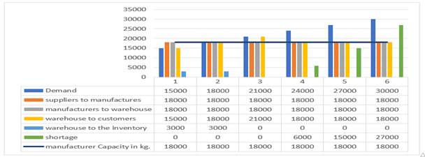
Figure 2 Production flow.

 

3.3. EFFECT OF THE MAXIMUM PERMISSIBLE DEVIATION ON SUPPLY CHAIN OBJECTIVES

While increasing the maximum permissible percent of deviation that decreases the profit values; the total cost will be increased as shown in Figure 3 and Figure 4. The total revenue remains constant at 10800000 $ in all cases. The OCSLs also does not changed and remain at 80% in all cases.

Figure 3

                                                                         

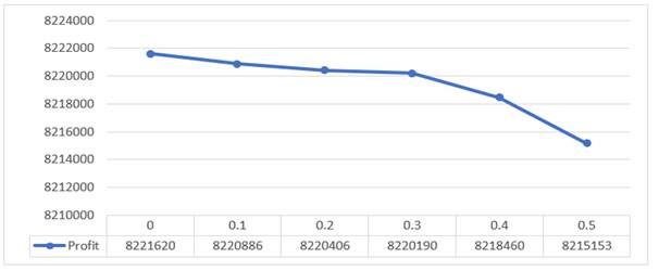
Figure 3 The resulted profit

 

Figure 4

                                                                        

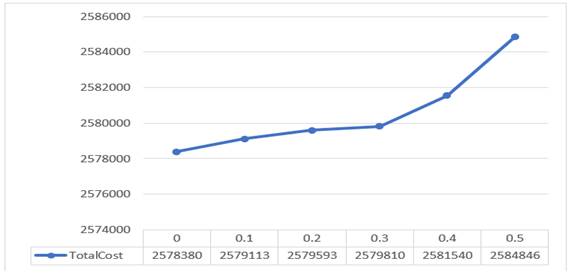
Figure 4 The resulted total cost

 

3.4. EFFECT OF OPTIMIZATION ORDER ON SC OBJECTIVES

In this section, the effect of changing solution priorities on target values at 0% and 30% diffraction values will be studied. Table 5 shows the different arrangements for the objectives, which are 6 arrangements.

In this section, it was noticed that changing of objectives aimed at optimization of profit with lees total cost, and better OCSLs, using deviation 0%, and 30%. At 0% deviation and changing of objectives; ended up by P-C-S, P-S-C, S-P-C and S-C-P as the best result. In deviation 0.3; ended up by P-C-S and S-C-P as the best result.

Table 5

Table 5 Objectives orders
Case	1	2	3	4	5	6
Order	P-C-S	P-S-C	S-P-C	S-C-P	C-P-S	C-S-P
P = profit, S = OCSLs, C = total cost

 

It appears from the results shown in Figure 5 and Figure 6 when the allowable deviation percentage is 0% that the acceptable arrangements are the ones that start with maximizing profit or maximizing the OCSL, as the results showed that giving priority to reducing costs negatively affects the rationality of the results and thus the performance of the supply chain.

Figure 5

                                                                          

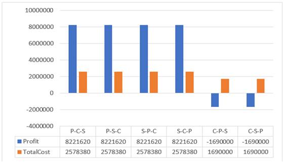
Figure 5 The resulted profit and total cost

 

Figure 6

                                                                          

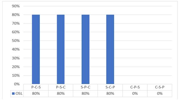
Figure 6 The resulted OCSLs

 

 

Also, it appears from the results shown in Figure 7 and Figure 8 when the allowable deviation percentage is 30% that the accepEq arrangements are the ones that start only with maximizing profit. or, as the results showed that giving priority to maximizing the OCSL or reducing costs negatively affects the rationality of the results and thus the performance of the supply chain.

It is clear from this study that it is very important to arrange the targets and to choose the maximum allowable deviation. Therefore, researchers recommend the necessity of experimenting with many values and arrangements and comparing them according to the priorities of decision-makers to choose the optimal design and planning for the supply chain as they see fit.

Figure 7

                                                                          

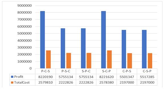
Figure 7 The resulted profit and total cost

 

Figure 8

                                                                          

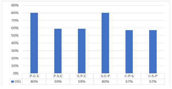
Figure 8 The resulted OCSLs

 

4. CONCLUSION AND RECOMMENDATIONS

 In this paper, a multi-objective sustainable supply chain network location-allocation model for perishable products has been developed to prevent the expiration of products considering the FIFO inventory policy to maximize the total profit of the network.

This model has successfully handled the problem of a multi-objective sustainable supply chain network location allocation for perishable products. It also helped in the prevention of product expiration by assuring that only the necessary quantities are produced without waste.

It is clear from this study that it is very important to arrange the targets and to choose the maximum allowable deviation. Therefore, researchers recommend the necessity of experimenting with many values and arrangements and comparing them according to the priorities of decision-makers to choose the optimal design and planning for the supply chain as they see fit. The ordering of objectives influences the factory's success as well as their allowable deviation.

It is recommended to develop the model to tackle the uncertainty in both demand and production capacity to produce more practical solutions.

 

CONFLICT OF INTERESTS

None. 

 

ACKNOWLEDGMENTS

None.

 

REFERENCES

Al-Ashhab, M. S. & Alanazi, F. (2022). Developing a multi-item, multi-product, and multi-period supply chain network design and planning model for perishable products. International Journal of Research - GRANTHAALAYAH, 10(4), 179-199.  

Al-Ashhab, M. S. (2016). An optimization model for multi-period multi-product multi-objective production planning. International Journal of Engineering & Technology IJET-IJENS, 16(01).

Al-Ashhab, M. S. Nabil, O. M., & Afia, N. H. (2021). Perishable products supply chain network design with sustainability. Indian Journal of Science and Technology, 14(9), 787-800. https://doi.org/10.17485/IJST/v14i9.24

Al-Ashhab, M.S. & Aldosari, N. (2022). Modelling and Solving a Sustainable, Robust Multi-Period Supply Chain Network for Perishable Products. INDIAN JOURNAL OF ENGINEERING, 19(51), 184-195.  

Arvan, M. Tavakkoli-Moghaddam, R. & Abdollahi, M. (2015). Designing a bi-objective and multi-product supply chain network for the supply of blood. Uncertain Supply Chain Management, 3(1), 57-68. https://doi.org/10.5267/j.uscm.2014.8.004

Chalmardi, M. K. & Camacho-Vallejo, J.-F. (2019). A bi-level programming model for sustainable supply chain network design that considers incentives for using cleaner technologies. Journal of Cleaner Production, (213), 1035-1050. https://doi.org/10.1016/j.jclepro.2018.12.197

Dai, Z. Aqlan, F. Zheng, X. & Gao, K. (2018). A location-inventory supply chain network model using two heuristic algorithms for perishable products with fuzzy constraints. Computers and Industrial Engineering, 338-352.  https://doi.org/10.1016/j.cie.2018.04.007

Diabat, A. Jabbarzadeh, A. & Khosrojerdi, A. (2019). A perishable product supply chain network design problem with reliability and disruption considerations. International Journal of Production Economics, (212), 125-138. https://doi.org/10.1016/j.ijpe.2018.09.018

Eskandari-Khanghahi, M. Tavakkoli-Moghaddam, R. Taleizadeh, A. A. & Amin, S. H. (2018). Designing and optimizing a sustainable supply chain network for a blood platelet bank under uncertainty. Engineering Applications of Artificial Intelligence, (71), 236-250. https://doi.org/10.1016/j.engappai.2018.03.004

GAMS (n.d.). GAMS Development Corp., General Algebraic Modeling System.  

Hajela, P. & Lin, C.-Y. (1992). Genetic search strategies in multicriterion optimal design. Structural Optimization, 4(2), 99-107. https://doi.org/10.1007/BF01759923

Herlina, L. (2022). An Integrated Production and Distribution Planning Model in Shrimp Agroindustry Supply Chain. 21(1), 1-19.

Holland, J.H. (1975). Adaptation in natural and artificial systems. Ann Arbor : University of Michigan Press.

Horn, J. Nafpliotis, N. & Goldberg, D. E. (1994). A niched Pareto genetic algorithm for multiobjective optimization. Proceedings of the First IEEE Conference on Evolutionary Computation. IEEE World Congress on Computational Intelligence, 82-87. https://doi.org/10.1109/ICEC.1994.350037

Isaloo, F. & Paydar, M. M. (2020). Optimizing a robust bi-objective supply chain network considering environmental aspects : a case study in plastic injection industry. International Journal of Management Science and Engineering Management, 15(1), 26-38. https://doi.org/10.1080/17509653.2019.1592720

Kocabay, S. & Alaçam, S. (2017). Algorithm Driven Design : Comparison of Single-Objective and Multi-Objective Genetic Algorithms in the Context of Housing Design.

Konak, A. Coit, D. W. & Smith, A. E. (2006). Multi-objective optimization using genetic algorithms : A tutorial. Reliability Engineering and System Safety, 91(9), 992-1007.  https://doi.org/10.1016/j.ress.2005.11.018

Patidar, R. Venkatesh, B. Pratap, S. & Daultani, Y. (2018). A Sustainable Vehicle Routing Problem for Indian Agri-Food Supply Chain Network Design. International Conference on Production and Operations Management Society (POMS), 1-5.  https://doi.org/10.1109/POMS.2018.8629450

Rashidi, S. Saghaei, A. Sadjadi, S. J. & Sadi-Nezhad, S. (2016). Optimizing supply chain network design with location-inventory decisions for perishable items : A Pareto-based MOEA approach. Scientia Iranica, 23(6), 3025-3045. https://doi.org/10.24200/sci.2016.4009

Rohmer, S. U. K. Gerdessen, J. C. & Claassen, G. D. H. (2019). Sustainable supply chain design in the food system with dietary considerations : A multi-objective analysis. European Journal of Operational Research, 273(3), 1149-1164. https://doi.org/10.1016/j.ejor.2018.09.006

Schaffer, J. D. (1985). Multiple objective optimization with vector evaluated genetic algorithms. Proceedings of the First International Conference on Genetic Algorithms and Their Applications.  

Trisna, T. Marimin, M. Arkeman, Y. & Sunarti, T. C. (2016). Multi-objective optimization for supply chain management problem : A literature review. Decision Science Letters, 5(2), 283-316.  https://doi.org/10.5267/j.dsl.2015.10.003

Validi, S. Bhattacharya, A. & Byrne, P. J. (2014). A case analysis of a sustainable food supply chain distribution system-A multi-objective approach. International Journal of Production Economics, (152), 71-87. https://doi.org/10.1016/j.ijpe.2014.02.003

Yakavenka, V. Mallidis, I. Vlachos, D. Iakovou, E. & Eleni, Z. (2020). Development of a multi-objective model for the design of sustainable supply chains : The case of perishable food products. Annals of Operations Research, 294(1), 593-621. https://doi.org/10.1007/s10479-019-03434-5

Zahiri, B. Zhuang, J. & Mohammadi, M. (2017). Toward an integrated sustainable-resilient supply chain : A pharmaceutical case study. Transportation Research Part E : Logistics and Transportation Review, (103), 109-142. https://doi.org/10.1016/j.tre.2017.04.009