1. INTRODUCTION
The iterative and recursive algorithms could be used to
solve matrix equations Wang (2007), Ding (2005), Xie (2010),
parameter estimation problems Li (2018), Li (2018), Liu (2010) and filtering issues Ma (2020). In parameter estimation approaches which are
recursive, the estimation of parameters can to be calculated
in an online framework Du
(2017), Wei
(2017). On the other hand,
the primary notion of the hierarchical algorithms is to update estimation of
the parameters by applying a set of data Ding
(2018), Ding
(2019), Sadeghi (2023). The hierarchical
parameter estimation approaches make adequate use of all output and input Data Li
(2020), Wang
(2020), and could enhance the
accuracy of estimation of parameters Li
(2020), Ding (2020) and convergence rate
of parameters Li
(2021), Chen
(2020).
Two-stage
algorithms have an enormous usage in the realm of parameter identification Sadeghi (2023), Sadeghi (2023) developed a two-stage
step-wise system identification approach for a class of nonlinear dynamic
systems Li
et al. (2006). In Raja
(2015), two-stage least mean
square adaptive methods relying on process of fractional signal were fostered
regarding CARMA systems. A two-stage neural network
algorithms related to ARMA model estimation by the use of a
simple mean called extended sample autocorrelation function is presented
Lee
(1994). In Bin
(2012), a two-stage method is
introduced regarding the system identification of an ARMAX model which
identifies ARX and MA part separately by bias-eliminated least squares
method and another basic method respectively. Also in Ding
(2020), a new two-stage
algorithm for estimating parameter of system is brought up but in this article
as a novelty, a CARMA system is discussed.
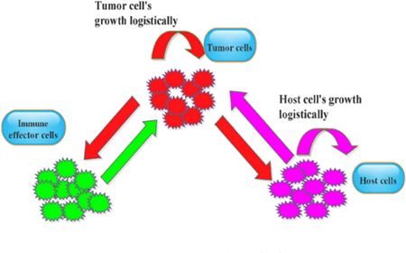
Having a suitable model for tumor system has become an
integral issue since the death rate of cancer has become considerable.
Accessing a suitable polynomial model for tumor can make the designing of a
controller for system much easier. In Pillis (2020),
a four population model is presented which contains tumor cells, host cells, drug
interaction, immune cells and a
controller based on optimization, which is used to satisfy the specific desire.
In Sweilam & AL-Mekhlafi (2018), an updated nonlinear
mathematical format of a general tumor beneath immune suppression is
discussed. The brought
up model in this paper is ruled by a fractional differential equations
system. Lobato (2016) presented another
model for tumor and in their works they aim to reach a
protocol of optimization for injection of drug to sick individuals having
cancer, by the making both of the cells having cancer and the drug
concentration which has been prescribed minimum Lobato (2016). Tumor model
presented in this last research is the basis of our study throughout the rest
of the paper.
Controlling a CARMA or ARMAX model system
has been the subject of a few papers and not much work has been done in this
field. For instance, In Chen
& Guo (1987), an optimal adaptive
control for ARMAX systems using a quadratic loss function is introduced.
In Li
(2021), abrupt faults in ARMAX
models have been taken into consideration and reliable control problem has been
studied. Multivariable system control is discussed in Osorio-Arteaga
(2020) where a robust
adaptive control is applied to ARMA and ARMAX structures of an
electric arc model. Furthermore, linear neural networks was
set as a study tool for adpative control of CARMA
systems Watanabe (1992).
In the following section, a nuance characteristic of the
system configuration regarding the CARMA configuration is brought up. Also,
section section 3 includes the mathematics of two
novel GI algorithm. Section 4 describes a specific tumor model. In section 5,
all the necessary simulations for showing the effectiveness of new algorithms
are illustrated by identifying a tumor model. Eventually, in the last section,
all the outcomes were derived.
2. System model: Carma systems
Take the introduced below CARMA system into
consideration:

Here u(t) is the succession of input of the system, y(t)
is the succession of output of the
system and  is a
succession of white noise with zero mean and variance
is a
succession of white noise with zero mean and variance  Also A(q), B(q) and c(q) are multinomial
in the monad backward variation agent [i.e.
Also A(q), B(q) and c(q) are multinomial
in the monad backward variation agent [i.e.  For simplicity in the rest of the paper, we
have the following notations: A =: X describes A is described as X; The
indication I (
For simplicity in the rest of the paper, we
have the following notations: A =: X describes A is described as X; The
indication I ( )
is an identity matrix with suitable dimensions (
)
is an identity matrix with suitable dimensions ( $1_{n}$
indicates a vector of n-dimensional column
which all components are 1. The superscript T indicates the transpose of
a matrix; the matrix
norm is described by
$1_{n}$
indicates a vector of n-dimensional column
which all components are 1. The superscript T indicates the transpose of
a matrix; the matrix
norm is described by  .
.
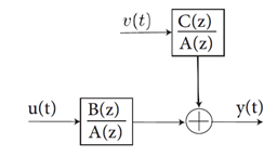
Now look at the CARMA system shown in Figure
\ref{fig.1}. We define A(q), B(q) and C(q) as polynomials of known orders  as
as
follows:


In a generic way, it is presumed that y(t) = 0, u(t) = 0
and  =
0 for t
=
0 for t  0. Take
  ,
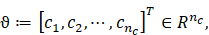
Consider the system parameter vectors:
,
Consider the system parameter vectors:

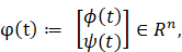
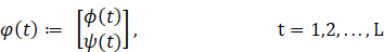
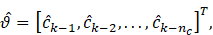
and the corresponding information vectors:


Based on the above definitions and equation (\ref{eq.1}),
we attain the the below parameter estimation
configuration:
 =
= ,
,
y(t)=  +
+
 +
+  , (2)
, (2)
y(t)=  + , (3)
3. Theory of identification and
control algorithms
3.1. Gradient based iterative
algorithms(GI)
We consider k=1,2,3,… as an
hierarchical variable  and
and
 as
the hierarchical identification of and
while k iteration has established. Beyond that
as
the hierarchical identification of and
while k iteration has established. Beyond that  is the biggest eigenvalue of the matrix of
symmetric format X.
is the biggest eigenvalue of the matrix of
symmetric format X.
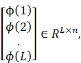
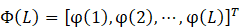
Now we take an array of data with length L which works
with the model introduced in. Here, we consider the vector of stacked output
data Y(L) and matrix of the stacked data
 like:
like:
Y(L):=
 :=
:=
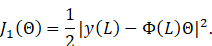
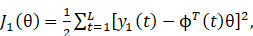
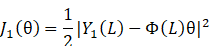
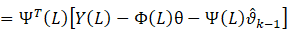
Now we define the static criterion function as follows:
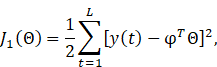
which can be equally described as:
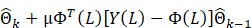
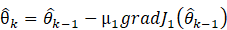
By taking advantage of negative gradient probe,
calculating the partial derivative of  regarding
  ,
we attain this iterative relation:
,
we attain this iterative relation:

=

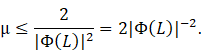
Here,  is a convergence factor or an iterative
step-size. To make sure about convergence of
is a convergence factor or an iterative
step-size. To make sure about convergence of  ,
all the eigenvalues of
,
all the eigenvalues of 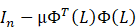 should be in the monad circle, so
  therefore as suitable conservative form of
  we have:
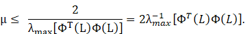
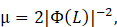
As to eschew calculating the intricate eigenvalues of a
matrix which is square and to decrease evaluation expense, the trace of matrix
is taken advantage of and capitalized on a different manner for picking up the
convergence rate:
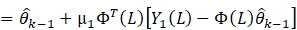
Now it is possible to attain the gradient based iterative
method for CARMA system presented in equation (1) with the following set
of equations:
 (4)
(4)
 (5)
(5)
 (6)
(6)
 (7)
(7)
 (8)
(8)
 (9)
(9)
 (10)
(10)
The steps of calculating from
equation (4)-(10) summarized as below:
1) Regarding
 set every variable to zero. Assume k = 1, take
the data length L (L
set every variable to zero. Assume k = 1, take
the data length L (L and
take the primary amounts,
and
take the primary amounts,  and the system identification precision
  .
.
2) Gather
all the input u(t) and output y(t) for t=1,2,…,L.
3) Attain
the vectors of information  by equation (9),
  by equation (10) and
  by equation (8).
4) Form
the vector of stacked output Y(L) regarding equation (6) and the matrix of
stacked information regarding equation (7), also pick up a large based on equation (5).
5) Upgrade
the parameter estimation vector $\hat{\Theta}{k}$ by
equation (\ref{eq.4}).
6) Contrast
with  .
If
.
If  extend
k in unit order and start from step 5. In all other respects, attain iteration
k and the system identification vector .
extend
k in unit order and start from step 5. In all other respects, attain iteration
k and the system identification vector .
3.2. Two-stage
Gradient based iterative algorithms (2S-GI)
Consider the CARMA model described in equation
(\ref{eq.2}).
First, we define these two imaginary output variables:
Afterwards by these definitions we have:
 (11)
(11)
 (12)
(12)
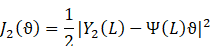
Take $L$ as data length. According to equation (11) and
(12), we define these two static criterion functions:
 (13)
(13)

Consider the vector of stacked output Y(L), vectors of the
stacked imaginary outputs  and
and  ,
and the matrices of stacked information
,
and the matrices of stacked information  and
and  are as follows:


Equations (13) and (14) can be equivalently written as:
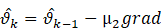
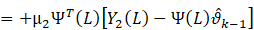
By taking advantage of the search of negative gradient to
make the criterion functions above minimum, we have:

=


To make sure about convergence of  and
and  all the eigenvalues of
  and
and  ,
should be in the unit circle, so we have:
,
should be in the unit circle, so we have:
Therefore, similar to GI algorithm as a conservative choice, we have
the following relation for  and
and 

In brief, we have
the following set of equations for 2S-GI algorithm:
 (15)
(15)
(16)


 (20)
(20)

(22)

 (24)
(24)
 (25)
(25)
The steps of attaining  and
and included in the 2S-GI approach from
equation (15)–(25) are brought up as follows:
included in the 2S-GI approach from
equation (15)–(25) are brought up as follows:
1) Regarding
 ,
put every parameter to 0. Imagine k=1 take the length of data as L (
,
put every parameter to 0. Imagine k=1 take the length of data as L (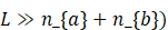 and set the initial values as:
 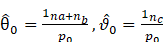 and the parameter estimation accuracy
2) Gather
all the input u(t) and output y(t) for t=1,2,…,L.
Attain the information vectors (22)
by equation (22) and (t)
by equation (23).
3) Build
the vector of stacked output Y(L) by (19) and the matrices of stacked
information and  by (20) and (21), calculate the convergence
factor and
by (20) and (21), calculate the convergence
factor and  regarding (16) and (18).
4) Update
the vectors of parameter approximation  by
by
(15) and (17).
5) Compare
 with
with
 and
and
 with
with  :If
:If
 +
+ >
,
extend k by $1$ and start from step 4. In all other respects attain iteration k
and the vectors of estimation of parameters and
.
>
,
extend k by $1$ and start from step 4. In all other respects attain iteration k
and the vectors of estimation of parameters and
.
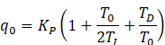
4. Control theory
In this part of the paper, theory of a ziegler
nichols PID controller for third order
processes introduced in (Bobal, 2006) is brought up. The control law which we
took advantage of is:
 (26)
(26)

Here  is the controller error. The feedback form of
control law is:
is the controller error. The feedback form of
control law is:
 (28)
(28)
Where  respectively are:

And we have:
 .
.
And  are ultimate period and ultimate gain
respectively.
are ultimate period and ultimate gain
respectively.
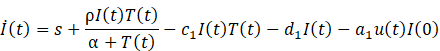
5. Tumor model
I indicate the immune cells number at time t, T denotes
the tumor cells number at time t, N describes the
normal (host) cells number at time t, and u is the plan of
control.\begin{figure}[h] \centering \includegraphics[width=.5\linewidth]{T-I-N.eps} \caption{Random tumor and
immune cells interactions.}
 ,
,

 .
.
Values of known parameters in above equations are listed
below Lobato (2016)
Parameter |
Values |
Parameter |
Values |

|

|

|
0.3 |

|
0.1 |

|
1 |

|
1 |

|
0.5 |

|
1 |

|
0.5 |

|
1 |

|
1 |

|
0.2 |

|
0.01 |

|
1.5 |

|
1 |
S |
0.33 |
|
|
Therefore, we yield: \begin{equation*} \begin{split}
 ,
,
 ,
,
 .
.
6. Simulations
6.1. Estimation of T(t)
In this paper, we aim to identify T(t) as the quantity of tumor cells at time t and I(t) as the quantity of immune
cells at time t, by presenting novel parameter estimation method. In
simulations assume  ,
,
 and
and
 .
In simulations,
.
In simulations, ,
,
 =1
and
=1
and  =1.
\subsection{Estimation of T(t)}
=1.
\subsection{Estimation of T(t)}
The CARMA model of T(t) as the output and u(t) as
the input is:


|
Table 1
Estimation Result for 
|
|
Algorithms
|
t=L
|

|

|

|
|
1000
|
-0.1005
|
-0.8864
|
-1.7053
|
|
GI
|
2000
|
-0.0970
|
-0.8816
|
-1.7751
|
|
3000
|
-0.0974
|
-0.8822
|
-1.7473
|
|
1000
|
-0.0976
|
-0.8835
|
-1.7570
|
|
2S-GI
|
2000
|
-0.0946
|
-0.8836
|
-1.7145
|
|
3000
|
-0.0921
|
-0.8797
|
-1.7161
|
|
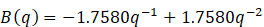
True value
|
|
-0.0862
|
-0.8937
|
-1.7580
|
|
Algorithms
|
t=L
|

|

|

|
|
1000
|
1.7859
|
-0.0460
|
-0.0020
|
|
GI
|
2000
|
1.7389
|
0.0229
|
0.0426
|
|
3000
|
1.7378
|
0.0231
|
0.0009
|
|
1000
|
1.7690
|
0.0019
|
-0.0030
|
|
2S-GI
|
2000
|
1.7380
|
0.0281
|
-0.0189
|
|
3000
|
1.7726
|
0.0455
|
-0.0485
|
|
|
1.7570
|
0.6264
|
-0.3459
|
|
Algorithms
|
t=L
|

|
|
1000
|
7.6604
|
|
GI
|
2000
|
6.8844
|
|
3000
|
6.4698
|
|
1000
|
6.8316
|
|
2S-GI
|
2000
|
6.2351
|
|
3000
|
5.7110
|
|
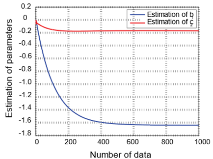
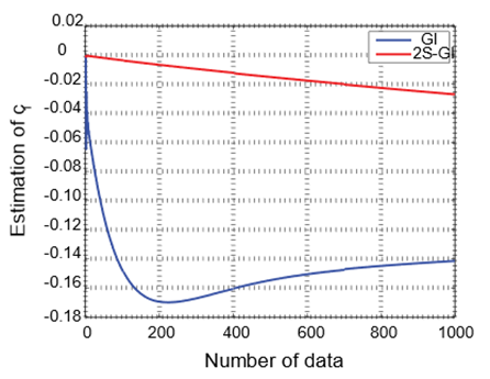
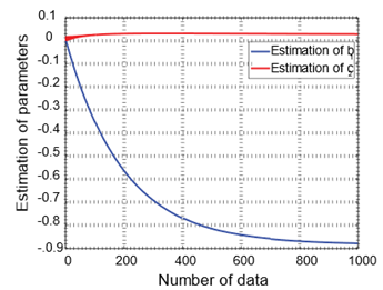
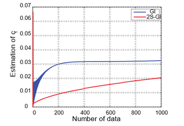
Estimation of  for
CARMA System with Variance for
CARMA System with Variance  and Number of Data L=1000 with 2S-GI Algorithm and Number of Data L=1000 with 2S-GI Algorithm
|
|
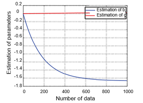
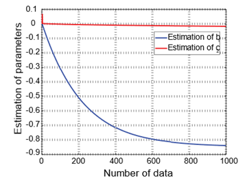
Estimation of  for
CARMA System with Variance and Number of Data L=1000 for
CARMA System with Variance and Number of Data L=1000
|
|
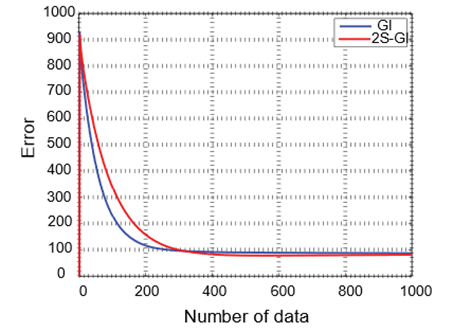
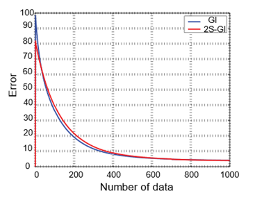
Estimation Error for CARMA System with Variance and Number
of Data L=1000
|
|
Table 2
Estimation Results for 
|
|
Algorithms
|
t=L
|

|
|

|
|
1000
|
-0.1182
|
0.8405
|
-1.6400
|
|
GI
|
2000
|
-0.1412
|
-0.8478
|
-1.7594
|
|
3000
|
-0.136
|
-0.8474
|
-1.7737
|
|
1000
|
-0.1379
|
-0.8400
|
-1.6632
|
|
2S-GI
|
2000
|
-0.1332
|
-0.8451
|
-1.6933
|
|
3000
|
-0.1270
|
-0.8465
|
-1.7573
|
|
True value
|
|
-0.0862
|
-0.8937
|
-1.7580
|
|
Algorithms
|
t=L
|

|

|

|
|
1000
|
1.8659
|
-0.1413
|
-0.1693
|
|
GI
|
2000
|
1.9069
|
0.0147
|
0.0319
|
|
3000
|
1.8679
|
0.0142
|
0.0082
|
|
1000
|
1.9208
|
-0.0274
|
0.0265
|
|
2S-GI
|
2000
|
1.8392
|
0.0123
|
-0.0094
|
|
3000
|
1.8060
|
0.0385
|
-0.0566
|
|
|
1.7570
|
0.6264
|
-0.3459
|
|
Algorithms
|
t=L
|

|
|
1000
|
8.6731
|
|
GI
|
2000
|
6.7497
|
|
3000
|
6.9010
|
|
1000
|
8.1050
|
|
2S-GI
|
2000
|
6.2351
|
|
3000
|
5.8114
|
6.2. Estimation of I(t)
The CARMA model of $I(t)$ as the output and u(t) as
the input is:


|
Table 3
Estimation Results for 
|
|
Algorithms
|
t=L
|
|
|
|
|
1000
|
-1.042
|
0.0541
|
0.8791
|
|
GI
|
2000
|
-0.9243
|
-0.0612
|
-0.8699
|
|
3000
|
-0.9436
|
-0.0405
|
-0.9078
|
|
1000
|
-0.9297
|
-0.05
|
-0.8541
|
|
2S-GI
|
2000
|
-0.941
|
-0.0471
|
-0.8699
|
|
3000
|
-0.127
|
-0.8465
|
-1.7573
|
|
True value
|
|
0.9499
|
-0.0345
|
-0.8921
|
|
Algorithms
|
t=L
|
|
|
|
|
1000
|
0.8782
|
-0.1586
|
0.0987
|
|
GI
|
2000
|
0.7725
|
0.0158
|
-0.0080
|
|
3000
|
0.7917
|
0.0165
|
0.0248
|
|
1000
|
0.7871
|
-0.0219
|
-0.0229
|
|
2S-GI
|
2000
|
0.7537
|
0.0324
|
0.0342
|
|
3000
|
0.7697
|
-0.0238
|
0.0200
|
|
|
1.7570
|
0.6264
|
-0.3459
|
|
Algorithms
|
t=L
|
|
|
1000
|
3.7344
|
|
GI
|
2000
|
3.0066
|
|
3000
|
2.3635
|
|
1000
|
2.9884
|
|
2S-GI
|
2000
|
2.1040
|
|
3000
|
1.9732
|
|
Table 4
Estimation Results for
|
|
Algorithms
|
t=L
|
|
|
|
|
1000
|
-0.9189
|
-0.0712
|
-0.8799
|
|
GI
|
2000
|
-0.8958
|
-0.0928
|
-0.9277
|
|
3000
|
-0.9008
|
-0.0857
|
-0.8848
|
|
1000
|
-0.9282
|
-0.0555
|
-0.8405
|
|
2S-GI
|
2000
|
-0.9542
|
-0.0366
|
-0.9301
|
|
3000
|
-0.1270
|
-0.8465
|
-1.7573
|
|
True value
|
|
-0.9175
|
-0.0647
|
-0.8817
|
|
Algorithms
|
t=L
|
|
|
|
|
1000
|
0.6899
|
-0.0324
|
0.0286
|
|
GI
|
2000
|
0.8068
|
0.0209
|
0.0159
|
|
3000
|
0.8065
|
-0.0254
|
-0.0163
|
|
1000
|
0.6995
|
0.0206
|
-0.0171
|
|
2S-GI
|
2000
|
0.8130
|
0.0207
|
-0.0189
|
|
3000
|
0.7981
|
0.0217
|
0.0273
|
|
|
1.7570
|
0.6264
|
-0.3459
|
|
Algorithms
|
t=L
|

|
|
1000
|
4.039
|
|
GI
|
2000
|
3.3538
|
|
3000
|
2.8344
|
|
1000
|
3.8944
|
|
2S-GI
|
2000
|
2.5776
|
|
3000
|
2.2446
|
7. Control of tumor models
The final goal of this research is to make the amount of tumor cells minimum, therefore we
take T(t)=0 as the desired output of the system. Based on control theory
introduced in the third section and the identified polynomial model of T(t),
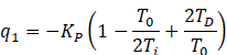
the ultimate period and ultimate gain is  and
and  Therefore
  and
and  and
and  .
.
The output and input of the feedback form is depicted in
the next two figures.
From tables and figures above, the below results are
derived:
·
The system identification errors of the GI and 2S-GI
approaches decrease as the data length increases.
·
2S-GI method, compared to GI method,
produces less error and therefore is more effective at estimating parameters.
·
As the noise to ratio signal rises, both
introduced algorithms produce a larger amount of error.
·
From figures, it is perceived that both
introduced algorithms converge at a final point and have a competent
convergence rate.
·
The introduced controller proved that, it is able to make the amount of tumor cells in a
specific period of time minimum.
8. Conclusion
In this contribution, mathematical theories and algorithms
of two
identification methods of GI and 2S-GI for CARMA systems were
developed. GI is an old method but 2S-GI is a
novel method which introduced in this paper. Furthermore, a tumor
model with one input and three outputs were presented by works of other
scholars. By means of introduced parameter estimation approaches, the model were identified. Above that, by taking advantage of a ziegler nichols PID
controller the amount of tumor cells were controlled and it was illustrated that the controller
could minimize amount of tumor cells in a specific
span of time. Also, the GI and 2S-GI algorithm showed that they both are able to estimate parameter of a polynomial CARMA
configuration in fast convergence rate and by producing an insignificant amount
of error.
CONFLICT OF INTERESTS
None.
ACKNOWLEDGMENTS
None.
REFERENCES
Bin, X. I. (2012). A Two-Stage ARMAX Identification Approach Based
on Bias-Eliminated Least Squares and Parameter Relationship Between MA Process
and Its Inverse. Acta Automática Sinica, 491-496. https://doi.org/10.1016/S1874-1029(11)60310-8
Bobál, V. E. (2006). Digital Self-Tuning Controllers: Algorithms,
Implementation and Applications. Springer Science & Business Media.
Chen,
H.-F., & Guo, L. (1987). Optimal Adaptive Control and Consistent
Parameter Estimates for ARMAX Model with Quadratic Cost. SIAM Journal on
Control and Optimization, 845-867. https://doi.org/10.1137/0325047
Chen, J. Q. (2020). Modified Kalman Filtering Based
Multi-Step-Length Gradient Iterative Algorithm for ARX Models with Random
Missing Outputs. Automatica. https://doi.org/10.1016/j.automatica.2020.109034
De Pillis, L. G. (2001). A Mathematical Tumor Model with Immune
Resistance and Drug Therapy: An Optimal Control Approach. Computational and
Mathematical Methods in Medicine, 79-100. https://doi.org/10.1080/10273660108833067
Ding,
F. A. (2005). Gradient Based Iterative Algorithms for Solving a Class of
Matrix Equations. IEEE Transactions on Automatic Control, 1216-1221. https://doi.org/10.1109/TAC.2005.852558
Ding,
F. E. (2019). Gradient-Based Iterative Parameter Estimation Algorithms
for Dynamical Systems from Observation Data. Mathematics. https://doi.org/10.3390/math7050428
Ding, F. E. (2020). Gradient Estimation Algorithms for the
Parameter Identification of Bilinear Systems using the Auxiliary Model. Journal
of Computational and Applied Mathematics. https://doi.org/10.1016/j.cam.2019.112575
Ding, F. E. (2020). Two-Stage Gradient-Based Iterative
Estimation Methods for Controlled Autoregressive Systems using the Measurement
Data. International Journal of Control, Automation and Systems, 886-896. https://doi.org/10.1007/s12555-019-0140-3
Ding, F. E. (2018). Iterative Parameter
Identification for Pseudo-Linear Systems with ARMA Noise Using the Filtering
Technique. IET Control Theory and Applications.
https://doi.org/10.1049/iet-cta.2017.0821
Du, D. E. (2017). A Novel Networked Online Recursive Identification
Method for Multivariable Systems with Incomplete Measurement Information. IEEE
Transactions on Signal and Information Processing over Networks, 744-759. https://doi.org/10.1109/TSIPN.2017.2662621
Ji, Z. E. (2020). An Attention-Driven Two-Stage Clustering Method
for Unsupervised Person Re-Identification. Computer Vision-ECCV 2020: 16th
European Conference. https://doi.org/10.1007/978-3-030-58604-1_2
Lee, J. K. (1994). A Two-Stage Neural Network Approach for ARMA
Model Identification with ESACF. Decision Support Systems. https://doi.org/10.1016/0167-9236(94)90019-1
Li, K., Peng, J.-X., & Bai, E.-W. (2006). A Two-Stage
Algorithm for Identification of Nonlinear Dynamic Systems. Automatica,
1189-1197. https://doi.org/10.1016/j.automatica.2006.03.004
Li,
L. Z. (2020). A Two-Stage Maximum a Posterior Probability Method for
Blind Identification of LDPC Codes. IEEE Signal Processing Letters, 111-115. https://doi.org/10.1109/LSP.2020.3047334
Li, M. A (2018). The Least Squares Based Iterative Algorithms
for Parameter Estimation of a Bilinear System with Autoregressive Noise Using
the Data Filtering Technique. Signal Processing, 23-34. https://doi.org/10.1016/j.sigpro.2018.01.012
Li, M. A. (2018). Auxiliary Model Based Least Squares Iterative
Algorithms for Parameter Estimation of Bilinear Systems using Interval-Varying
Measurements. IEEE Access, 21518-21529. https://doi.org/10.1109/ACCESS.2018.2794396
Li, M. A. (2020). Maximum Likelihood Least Squares Based
Iterative Estimation for a Class of Bilinear Systems using the Data Filtering
Technique. International Journal of Control, Automation and Systems, 1581-1592.
https://doi.org/10.1007/s12555-019-0191-5
Li,
M. A. (2021). Maximum Likelihood Hierarchical Least Squares-Based
Iterative Identification for Dual-Rate Stochastic Systems. International
Journal of Adaptive Control and Signal Processing, 240-261. https://doi.org/10.1002/acs.3203
Liu, Y. D. (2010). Least Squares Based Iterative Algorithms for
Identifying Box-Jenkins Models with Finite Measurement Data. 1458-1467. https://doi.org/10.1016/j.dsp.2010.01.004
Lobato, F. S. (2016). Determination of an Optimal Control
Strategy for Drug Administration in Tumor Treatment using Multi-Objective
Optimization Differential Evolution. Computer Methods and Programs in
Biomedicine, 51-61. https://doi.org/10.1016/j.cmpb.2016.04.004
Ma, H. E. (2020). Partially-Coupled Gradient-Based Iterative
Algorithms for Multivariable Output-Error-Like Systems with Autoregressive
Moving Average Noises. IET Control Theory and Applications, 2613-2627. https://doi.org/10.1049/iet-cta.2019.1027
Osorio-Arteaga, F. J.-D. (2020). Robust
Multivariable Adaptive Control of Time-Varying Systems. IAENG International
Journal of Computer Science, 605-612.
Raja, M. A. (2015). Two-Stage Fractional Least Mean Square
Identification Algorithm for Parameter Estimation of CARMA Systems. Signal
Processing, 327-339. https://doi.org/10.1016/j.sigpro.2014.06.015
Sadeghi, K. H. (2023). Efficient
Identification Algorithm for Controlling Multivariable Tumor Models:
Gradient-Based and Two-Stage Method. Advanced Mathematical
Models and Applications, 8(2), 185-198.
Sadeghi, K. H. (2023). Multi-Innovation Iterative
Identification Algorithms for CARMA Tumor Models. International Review on
Modelling and Simulation. https://doi.org/10.15866/iremos.v16i2.23270
Sadeghi, K. H. (2023). Utilizing ARMA Models for System
Identification in Stirred Tank Heater: Different Approaches. Computing Open. https://doi.org/10.1142/S2972370123300030
Sweilam,
N. H., & AL-Mekhlafi, S. M. (2018). Optimal Control for a Nonlinear
Mathematical Model of Tumor Under Immune Suppression: A Numerical Approach.
Optimal Control Applications and Methods, 1581-1596. https://doi.org/10.1002/oca.2427
Wang,
L. E. (2020). Decomposition-Based Multiinnovation Gradient
Identification Algorithms for a Special Bilinear System Based on its
Input-Output Representation. International Journal of Robust and Nonlinear
Control, 3607-3623. https://doi.org/10.1002/rnc.4959
Wang, M. X. (2007). "Iterative Algorithms for Solving the
Matrix Equation AXB+ CXTD= E.". Applied Mathematics and Computation, 622-629.
Watanabe, K. T. (1992). An Adaptive Control for CARMA
Systems Using Linear Neural Networks. International Journal of Control,
483-497. https://doi.org/10.1080/00207179208934324
Wei,
Z. E. (2017). Online Model Identification and State-of-Charge Estimate
for Lithium-Ion Battery with a Recursive Total Least Squares-Based Observer.
IEEE Transactions on Industrial Electronics,
1336-1346.
Xie, L. Y. (2010). Gradient Based and Least Squares Based Iterative
Algorithms for Matrix Equations AXB+ CXTD= F. Applied Mathematics and
Computation, 2191-2199. https://doi.org/10.1016/j.amc.2010.07.019