Machine Learning Models for Extrapolative Analytics as a Panacea for Business Intelligence Decisions

 

Richmond Adebiaye ¹, Mohammed Alshami ², Theophilus Owusu ³

 

¹ PhD, Department of Informatics& Engineering Systems, College of Arts & Sciences, University of South Carolina Upstate, USA

² College of Economics and Management, Al Qasimia University, UAE

³ The Graduate School, College of Business, Keiser University, FL, United States

 

1. INTRODUCTION

The importance of business intelligence (BI) to support and facilitate better business decisions cannot be over-emphasized. BI concept is defined as a combination of business analytics, data visualization, data infrastructure and tools, process, politics, culture, technologies, and best practices to help organizations make more data-driven decisions What is Business Intelligence? Your Guide to BI and Why it Matters. (2021). Therefore, it is imperative that strategic planning and value should be clearly defined by an organization to include both political and cultural aspects before decisions are made on BI technology. The benefits of implementing BI are “improved decision making, an increase in revenue, an improvement in customer satisfaction, and an increase in market share Hočevar and Jaklič (2010)”. Business intelligence (BI is much more than specific but rather “an umbrella term that includes processes and methods of collecting, storing, and analyzing data from business operations or activities to optimize performance” Adebiaye and Conner (2015). This collaborative definition quickly evolved into more processes and activities to help improve performance over the past few years. BI has evolved to include data mining, reporting, performance metrics and benchmarking, descriptive analytics, querying, statistical analysis, data visualization, visual analysis, and data reparation.

BI can help the auto dealership sales force by providing visualizations of the sales cycle, in-depth conversion rates analytics, as well as total revenue analysis. Invariably, BI can help the sales team in identifying what’s working as well as points of failure which can result in dramatically improved sales performances. Implementing BI in an auto dealership also provides invaluable insights into their financial data, stock control, and revenue decisions. With accumulated data based on daily routine activities in the business, BI could help quantify the elements related to “data collection, data governance, data storage, data analysis, and an application of data mining which eventually could result in useful information to support a decision-making process Foley and Guillemette (2010)”. Daily decisions on purchasing activities, business offers, business strategies, and stock control would be a panacea that enables the auto dealership to have better revenue, lower costs, and achieve its organizational goals. 

In this study, the application of data and BI concept mining are presented from a certified used car company in Texas. The core of the decision-making determinant is to determine if the fulfillment and inventory acquisition processes of their products and services are solely on the subjective judgment of the general manager or the supervisor. This decision-making process criteria taken into consideration include the relevant data in the auto dealership that relates to vehicle inventories that were acquired within a specific time. The dataset representing the criteria was analyzed to provide more insightful ways of creating a data-driven decision-making process. Bi method of data mining approach was utilized for data collection based on the motivation which relies on the operational policy of the company.

 

2. The objective of the Study

The objective of this study is to test the effectiveness of the decision-making process of the auto industry in both the fulfillment and acquisition of products. The objective is to apply business intelligence approaches and machine learning models to historical data to determine an improved sales duration on each vehicle.

 

3. Related Works and Literature Review

Statistics of sales of certified used vehicles in the United States were 40.8 million units in 2019. It was recorded that within this same year, approximately 17 million new automobiles were sold in the US Statista (2021).  This indicates that a significant percentage of these vehicles are sold in the US (more so than anywhere else in the world), a strong presence that the automotive market is worth annual tens of billions of dollars. Researchers have used different methods to predict the price of certified used vehicles and most of which were adopted for this study. Other related works like “Adaptive Neuro-Fuzzy System Wu et al. (2009), Linear Regression (Oprea (2011), Pudaruth (2014)), Naive Bayes (Oprea (2011), Pudaruth (2014)), Decision Tree (Oprea (2011), Pudaruth (2014)), Artificial Neural Networks (Peerun et al. (2015); Sun et al. (2017), Thai et al. (2019), and Random Forest (Chen et al. (2017))” are among many methods used in pricing used cars. This study aimed to determine and predict the timeline for the sale of a car at the auto dealership and the acceptability of that duration of time. The accuracy and acceptability of this determination and the prediction using this model would enhance the decision-making processes of the auto dealership Statista (2021).

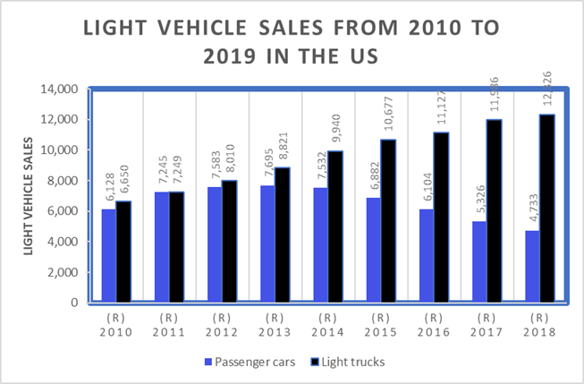
Figure 1

Figure 1 Graphical Representation of Vehicle Sales in the US from 2010 to 2019 (Statista, 2020)

 

Business intelligence (BI) capabilities regenerate into a strong competition. This is peculiarly higher in the automotive industry throughout the world. It has been estimated that global sales of automobiles or motor vehicles exceeded 1.175 billion yearly which is about one-seventh of the total world’s population Sousanis (2011). This creates strong employment and brand loyalty among consumers and is the most important and demanding field in the world economy Anderson (2018). Due to tremendous growth in the automotive industry, several emerging technologies were considered to enhance competition among automotive brands Anderson (2018). The competition transformed the automobile manufacturers to focus on “sustainable development strategies that are cost-effective and consistent with companies’ objectives” Farris et al. (2016).     BI concept feeds on different tools, applications, technologies, and practices that collect organizational raw data and analyze it. Subsequently, it is presented in an actionable business information form that can be used by a car dealer to make better decisions and also to find major changes in the environment of business (Chen et al. (2017)). Auto dealers can also BI methods to keep up with the shifting trends in trades. This enables dealers to adapt in response to trends and the change in the business environment quickly ("What is Business Intelligence & How it boosts Auto Dealership? | FrogData", 2019).

The Business intelligence capabilities and analytics of data have grown sufficiently to facilitate data access ability in recent years so, it helps the dealer employees to have access to reports and metrics without having to wait for accessibility approval to data. It also removes speculation needs Chen et al. (2017). This is because, in most auto dealerships, there's a high chance that instincts or estimations are being used by the top management to make decisions that put the reputation of the dealership at stake. instances have also been found where a structured data framework could be missing for vehicle dealerships to create effective business decisions Zetu and Miller (2010). Therefore, business intelligence and data analytics give the dealership insights based on data that is relevant and therefore enable better decision-making. It also helps in the prediction of changing trends that reduce the risks that might be faced in a failure of upkeep Farris et al. (2016). Finally BI is also crucial to give insights into customer buying patterns and behaviors. These actionable insights facilitate the gain of higher profits and new customers. Auto dealers dealing in used cars can take appropriate steps with these data analytics and save time Anderson (2018). In today’s global automotive market, customer orientation and services, pre-purchase research, experience with the dealer’s sales staff, experience driving the vehicle, service department, and interaction are some of the determinants for sales and brand ownership decisions by the dealers Zetu and Miller (2010).

The higher speed and better performance with a limited sample number (thousands) make the Support vector machine (SVM) a preferred machine learning algorithm for text classification issues. Support Vector Machine is a supervised algorithm learning-by-example paradigm spanning a broad range of classification, regression, and density estimation problems” Herbrich (2016). This represents a systematic approach based on statistical learning theory that “combines ideas from various scientific branches such as mathematical programming, exploiting the quadratic programming for convex optimization, functional analysis, indicating adequate methods for kernel representations, and machine learning theory, exploring the large maximum classifiers concept” Nechyba and XU (2017). The prediction of car sales is an important and rewarding problem in current times. The report generated percentage revenue from cars registered between 2009-2010 and 2015-16 witnessed a spectacular increase of 34% Listani (2019). The number of cars in 2016 reached 25,634,824. With a rise in new technologies and advancements, the sale of cars and the scope of this study will likely see growth.

 

4. Data Collection

The data of 243 cars purchased within the past year were obtained from a used Toyota dealership in Texas, McKinney. This data showed that 50% of the automobiles were sold way later than the acceptable duration of 30 days as desired by the company. This study aims to improve the accuracy that revolves around decision-making with the use of historical data so that more cars can be resold in an acceptable duration of time. To determine the data extraction criteria, an appraised function was established, and an appraiser then records an assessment using a data form. The Appraisal form contains all aspects of auto criteria considered important for auto dealership transactions. In total, 45 aspects of an auto feature/criteria were assessed.  The considered aspects of assessments are:

·        Document - Car registration forms, Car Titles, Car manuals, etc.

·        Exterior Car Accessories – Bumpers, Motor Hood, Wipers, etc.

 

·        Interior Car Accessories – Car Seats, Seat belts, Entertainment systems, etc.

·        Motor systems - Motor (engine, transmission), etc.

·        Motor parts – Wirings, coupling, Fenders, Sensors, Rims, Tires, side mirrors, etc.

In all aspects established for assessments, the appraiser needs to analyze the level the car satisfies in a particular aspect. Certain aspects may have binary levels, e.g., for the Manual Book aspect, the levels are “available” and “not available” –which means that a new purchase has to be made by the company. They may be more than two levels, e.g., for audio systems, there are three levels, i.e., “functions well”, “needs to be repaired”, and “broken” –which means a new purchase will be made by the company. Once the appraisal form reaches its completion it is then given to the supervisor which takes the purchasing decisions for the assessed car. An assessment of 543 cars has been done in these 45 aspects and it also is the data set in this study. The company decided to purchase these cars based on the assessment done by the appraisers. Each car's time lifespan or duration in the stock was also recorded through the data until it was sold.

 

5. Methodology

The computation of data dimensions as well as data records for data mining was presented to handle complex data structures to build an inferential model. Thus, the methodology utilized the application of a Contingency Table as a standard algorithm concept in the application of the data mining methods of BI in this study. For a data processing plan in this study, it is imperative to determine which independent variables to be included in our model. Referencing the BI concept and data mining context, a logical operational and scientific method was deployed in the form of the contingency table. The contingency table helps determine if there is an association between two categorical variables. This technique was implemented to evaluate relationships between the number of attempts in programming exercises and the final exam performance of the students Ahadi (2017). Other researchers like Das et al. (2018), Giudici and Passerone (2002), and Zytkow and Gupta (2001) used machine learning techniques to find associations in the domain of transport safety, assess the relationship between consumer behaviors, and identify patient condition patterns respectively in their studies. Accurately predicting the sale price of a car is a tedious yet rewarding action. Large numbers of features and records make the analysis very complex Sigh et al. (2017). The said parameter is dependent on many factors that make up the characteristics list of the product. The most important ones are usually the mileage of the car, its make (and model), the origin of the car (the original country of the manufacturer), and its horsepower.

 

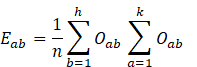
The Contingency Table Classifications

In line with the probability and statistics concept of two-event dependency, a contingency table technique was applied in the computation of expected frequencies of a table cell defined by the intersection of a row say a, and column b. The expected frequency of cell  is defined as  while the observed data point is defined as . The columns and rows for the contingency table are assumed independent of each other and the number of row levels is defined as  and column levels as .

 

 

Equation one: Expected frequency

 

 

Equation 2:  Chi-square tests for Association.

 

          

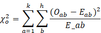
The chi-square test for Association defined by equation two above is applied to investigate the association between the rows and the columns of a contingency table. The critical values from the s statistical table are compared to the computed chi-square value to give a decision. Additionally, the p-value computed from the chi-square test can also be applied to achieve a final decision.

Null Hypothesis: Columns, Rows are independent (No association)

Alternative Hypothesis: Columns, Rows are dependent (There is an association)

 

Business Intelligence Implementation Equation Models Applied

Computation of data mining method applied with their formulas are as detailed below:

Decision Tree (CART)

A decision tree is computed to relatively start at the root node of the training dataset presented.  In machine learning, a decision tree is a tool for decision-making that employs tree-like models in evaluating the best decision based on some input data. Generally, it is categorized under the classification models since it classifies data points into distinctive classes based on some defined conditions. The decision tree begins splitting the data from a feature say k that has the highest information gain. The data is split into subsets say  . In this study, we consider a decision tree model that splits the data into two subsets  The two data subsets can be split again based on a parent node to obtain child nodes. The data split on the left contains the observations  while the data on the right contains the observations. The assumption was that “if all data in a node have the same label, then the node is not split any further. Otherwise, the node is split based on the best attribute (i.e., feature).  In the CART algorithm, the criterion to select the best attribute is ‘Maximum Gini gain’ Rutkowski et al. (2014)”.

The Gini impurity index measures the likelihood of an incorrectly labeled element obtained from the dataset given the element was randomly labeled according to the parent distribution. In other words, the score measures the proportion of the dataset say D that contains observations falling on the left () and the observation on the right ().

 

Equation 3: The formula is defined as:

 

. denotes the subsets of the data D that contains data with the label  . The waited Gini score is defined as

 

Equation 4: 

 

Random Forest (RF)

RF uses the majority vote from a set of decision trees to classify unlabeled data. Each tree is constructed by a data set that is sampled from the original training data set with replacement. In a tree, “to split a node, a set of random features are considered. The set of random features is a subset of the set of all features in the original training data set” Oshiro et al. (2012) .

 

K-Nearest Neighbors

An example of a supervised learning model is the k-nearest neighbors. This model takes in random data and outputs data classes that have similar characteristics Oshiro et al. (2012). Based on the Euclidean, the models classify unlabeled data points to the class of the nearest  neighbors.

 

Equation 5:  Given an  dimensional datasets, the Euclidean distance  is constructed as per the formula:

Based on the  smallest distances computed, new data points are given the label of the most frequent label among the selected  smallest distances.

 

Logistic Regression

Consequentially, Logistic Regression is better suited to describe the relationships between predictor variables. This could be “categorical or continuous, and a categorical outcome variable Peng et al. (2002)”. This usually models the natural log of the odds in the computational “outcome of the interest as a linear function of the predictor variables, i.e., features”. In this study, logistic regression models handle prediction cases where the dependent variable (y) is categorical and binary structure. The explanatory variables can be both continuous and categorical Peng et al. (2002). The odds of the outcome in the reference class are modeled using the logistic model.

 

Equation 6: The explanatory variables  contains the features of the models that determine the label value in the dependent variable  . The model takes the form.

 

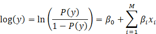
both  are the model parameters that need to be estimated.

 

Support Vector Machine (SVM)

The objective of the Support Vector Regression Model or Machine (SVM) here is to find a hyperplane (wx-t) that sorts data in the training dataset based on their labels. For instance, data labeled 1 on one side of the hyperplane are labeled -1 on the other side Peng et al. (2002). Additionally, the chosen hyperplane must ensure the distance between the hyperplane and date instances (support vectors) is maximized. Support vector machine classifies the data into ‘classes’ by finding a hyperplane separating the data points. the model randomly chooses support vectors and maximizes the distance between them to obtain the data classes Peng et al. (2002). For this, we considered a hyperplane in a two-dimensional space () separating the two data classes. The vector  contains the coefficients of the hyperplanes.

 

Equation 7: The feature vector is denoted as  and the data label is denoted as

 

      In the case where the data is not “linearly separable, a soft SVM” model is introduced. This model allows data points to close the hyperplane and the defined margin. A penalty is applied due to misclassification tolerated by the model.

 

Equation 8:  The parameter G regulates the effect on the objective function (Rish, 2001).

 

 

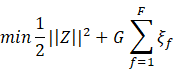
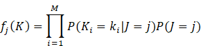
Naïve Bayes (NB)

The Naïve Bayes classification model is derived from the Bayes theorem and the conditional probability events. The idea behind Bayes classification is to classify a data point to a particular class or category if given some observation. Based on prior knowledge, the probability that a data point belongs to a certain class is generated Rutkowski et al. (2014). Consider an M-dimensional vector K containing the explanatory variables and label feature variable E. The data point is classified as the class with the highest .

 

Equation 9: The probability  can therefore be computed from the training dataset for each explanatory variable. This results in probability  based on the labels of the training dataset allowing the classifier to take this form:

 

Classification Models Performance Metrics

In Table 1 below, the performance of a model was summarized and illustrated using a confusion matrix based on the binary classification problem.

Table 1

Table 1 Confusion Matrix Illustrated and Classified
	“Actual Label: Positive”	“Actual Label: Negative”
“Predicted Label: Positive”	“TP() (True Positive)”	“FP() (False Positive)
“Predicted Label: Negative”	“FN() (False Negative)”	TN() (False Negative)”

          

Figure 2

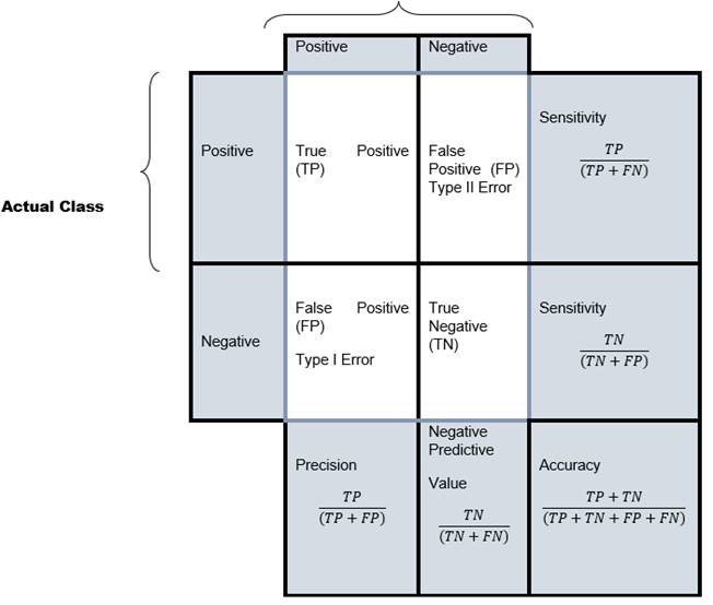
Figure 2 Confusion Matrix with Advanced Classification Metrics Science (2019)

 

The above figure illustration shows how the metrics used in this study are defined using machine learning based on the implementation of four performance metrics which are, i.e., “Precision, Recall, F1-Score, and Accuracy matrices. Caruana and Niculescu-Mizil (2004), Abidin et al. (2020)”, otherwise referred to as the four outputs in the “confusion matrix to determine the performance classifier. It contains the actual and predicted classifications. True Positive (TP) represents the number of correct predictions”, while False Negative is the number of incorrect predictions. On the other hand, False Positive (FP) is the number of incorrect predictions of a negative class incorrectly identified as positive while True Negative (TN) represents the number of correct predictions of a negative class correctly identified as negative.

Sensitivity is the actual “True Positive Rate or Recall” and represents the measure of positive examples labeled as positive by the classifier, while Specificity is the “True Negative Rate” which is a measure of negative examples labeled as negative by the classifier. Finally, Precision is the ratio of predicted positive examples to the “total number of correctly classified positive examples and the total number”. Accuracy is the proportion of the total number of correct predictions. F1 Score is the weighted average of the rate/recall (sensitivity) and precision. Science (2019)

F1 Score = 2 x Precision x Recall / Precision + Recall Science (2019)

 

Therefore, for this study, Accuracy metrics that measure the model are computed as “(TP + TN) / (TP + FP + FN + TN”). Model precision represents the “proportion of data classified as positive” and is computed as TP / (TP + FP) Science (2019). While ‘Recall’, “computes the proportion of data that are labeled as positive being classified as positive, i.e., TP / (TP + FN)”.

 

Model’s Descriptive Statistics Computation on Predictive Variables

Table 2

Table 2 Descriptive Statistics
Variables	N	Minimum	Maximum	Mean	Std. Deviation	Variance
Sales_in_thousands	167	0.11	680.561	61.99808	78.029422	4628.002
__year_resale_value	131	6.16	66.55	19.07298	12.453384	131.18
Price_in_thousands	165	9.235	85.5	27.39075	14.351653	205.97
Engine_size	166	1	8	3.061	1.0447	1.091
Horsepower	166	55	450	185.95	56.7	3214.926
Wheelbase	166	92.6	138.7	117.487	8.6413	58.39
Width	166	62.6	79.9	71.15	3.4519	11.915
Length	166	149.4	224.5	187.344	13.4318	180.412
Curb_weight	165	1.995	5.572	3.37803	0.630502	0.398
Fuel_capacity	166	10.3	32	17.952	3.8879	15.116
Fuel_efficiency	164	15	45	23.84	4.283	18.342
Power_perf_factor	165	23.27627233	188.144323	77.0435912	25.1426641	632.154

 

Table 2 above shows the descriptive of car sales data from this table we noticed that some variables contain 157 observations some contain 156 observations and year resale values contain 121 observations all other observations are missing in the data. Minimum and maximum values show the maximum and minimum points of each variable. The mean of the data shows how data lies about their center and variance and standard deviation tell us about how data separate around the center of data.

 

Testing the Impact of Variables on Car Sales

Multiple linear regression: MLR is a statistical technique that uses several explanatory variables to predict the outcome of a response variable. The “goal of multiple linear regression is to model the linear relationship between the explanatory (independent) variables and response (dependent) variables” Science (2019). MLR is the “extension of ordinary least-squares (OLS) regression because it involves more than one explanatory variable”. To test which of the variables has a significant impact on car sales, a multiple linear regression was applied.

 

Assumptions

For applying multiple regression analysis first need to check its assumptions. Assumptions are as follows:

1)     Linearity

2)     Homoscedasticity

3)     Normality

 

Normality

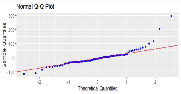
Normality checked by Q-Q plot. Graph 1 shows that the dependent variable is almost normally distributed there is no issue with it. So, the normality assumption is met.

 

Linearity and Homoscedasticity

  

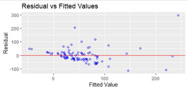
     To check the linearity, the graph between residual and fitted values above graph shows that there is a linear relationship between both the fitted line and residual. Also, these points are scattered so there is no homoscedasticity in it.

 

Multiple Regression Output

 

The model is computed as follow

 

Most of the predictors are not significantly related to the dependent variable so will remove all insignificant variables from the model to get more precise results.

 

6. Results and Discussions

Feature Selection

The intent would be to have listed cars resold in 30 days or less. The data provided supported the decision-making with an assessment concerning 45 aspect ratio classifications in a vehicle. However, when the number of features is compared to the number of instances of data, it became evident that the number of features represented is higher in the data mining methods for the performance of each aspect classification. Therefore, the use of a contingency table is to find this significant association of a car/vehicle with the success that a vehicle can be sold within an acceptable duration. The process was depicted using feature selection. For a contingency table construction, the categorization of each used car was, therefore, based on their duration in stock - which should be “within the acceptable duration and not more than 30 days”. A variable feature of each vehicle is classified into levels as “available or not available” in the car registration form. Table 3 is subsequently populated with the frequency of data on the “intersection of the column and row”. In retrospect, the table shows how 83 vehicles were purchased without a valid car registration form but were still sold within 30 days.

Table 3 

Table 3 Contingency Table for Registration Document and Duration in the Stock
	Stock Duration
Car Registration Form	≤ 30 days	> 30 days
Not available	72	65
Available	198	208

 

Contingency Table data becomes the “input for performing hypothesis tests on all pairs of car aspects and the duration in the stock”. On a significance level of 0.05, we obtain 12 variable vehicle features that have a “significant association with the duration in stock” Science (2019). These 12 vehicle variable features are used for the subsequent data mining applications. The features are represented in Table 4 with their values.

Table 4

Table 4 Selected Features and the Possible Values
No	Feature	Possible Values
1	Vehicle Registration Form	0                 = valid 1                 = certifiedVehicle() to be re-registered
2	Vehicle Manuals	0                 = Manual book available 1                 = vehicleManual() to purchase
3	Spare keys	0                 = Spare key functional 1                 = Spare key: common need 2                 = Spare key: customer requests
4	Bumpers and condition	0                 = Front bumper’s condition 1                 = needs repairs 2                 = needs replacements
5	Fenders’ conditions	0                 = Good fender’s condition 1                 = needs repairs 2                 = needs replacements
6	Doors conditions	0                 = All doors in good condition 1                 = One door panel needs repairs/replacement 2                = Two door panels need repairs/replacement 3                 = Three door panels need repairs/replacement 4                 = Four door panels need repairs/replacement
7	Transmission condition	0                 = Transmission functioning 1                = Transmission needs repairs or replacement
8	Exhaust systems	0                 = Exhaust systems with no issues 1                 = requires repairs/replacement
9	windshield condition	0                 = Windshield in good condition 1                = Front windshield to be replaced 2                = Both windshields to be replaced
10	Roof Top condition	0             = Roof Top well-conditioned 1             = Top roof protector broken 2             = Top roof partially damaged 3             = 100% needs to be replaced
11	Dents and Minor condition	0             = Exterior and frames in good condition 1             = 50% exterior parts to be replaced or repaired 2             = The entire exterior needs all over repairs
12	Tires and rims condition	0             = All tires and rims in great conditions 1             = One tire needs replacement 2             = Two tires need replacement 3             = Three tires need replacement 4             = All tires need replacement 5             = Rims to be replaced

 

Model Classification and Results

There are 243 cars in each data set. The labeling is done with either one or 0 indicating if it was sold in 30 days or less. These levels are balanced, i.e., 50.28% are labeled as one that is further divided into test and Training datasets randomly, which include 20% and 80% proportions respectively. Data mining methods to find parameters that can be tuned are applied through cross-validation in the data set trained using the “60-20-20 rule of thumb in machine learning Moews et al. (2019)”, including folds for cross-validation being classified. In each fold of cross-validation, data used for Training was 60% and data for testing was 20%. The best parameter set was “selected based on the highest average F1 score in all folds”. The model of final classification was fitted with the selected parameters in the training data set.  Different values of parameters are evaluated for different methods shown in Table 5. If there were more than one set of parameters, there is a pairing of parameter values for a particular run. For example, in Multinomial Logistic Regression, regularization strength in the first trial was off by 0.5, and the ‘lbfgs’ solver for vile regularization strength was 0.5. The Lib linear solver was used on the second trial, and in the same order. The parameter set for the highest average F1 score was in the cross-validation increased four-folds. For the naive bayes evaluation method, there were no parameters for the session. In all, the Training utilized 80% of the data set that includes the validation and training sets without the performance of cross-validation.

Table 5

Table 5 Evaluated Parameters in each Machine Learning Method
Data Mining Method	Parameters
“Decision Tree”	“Maximum depth = [2, 10]”
“Random Forest”	“Maximum depth = [2, 10]”
“k-Nearest Neighbors”	“k = [1, 326]”
“Logistic Regression”	“Regularization strength (C) = {0.5, 1, 2, 5} Solver = {lbfgs, liblinear, sag, saga, newton-cg}”
SVM	“Regularization strength (C)= {0.5, 1, 2, 5} Kernel type = {linear, poly, rbf, sigmoid}”

 

 

The methods identified in Table 6 are “sorted from the highest Test F1-Score”. The data mining implementations are performed using Python, using the ‘sklearn’ package.

Table 6

Table 6 Evaluated Parameters in each Machine Learning Method
Method (Selected Parameters)	Cross-validation/Training F1-Score	Test F1- Score (%)	Test Precision (%)	Test Recall (%)	Test Accuracy (%)
Support Vector   Machine (SVM) (C = 2, Kernel = poly)	84.35	84.42	71.94	91.76	79.54
Decision Tree (maximum depth = 7)	81.33	81.30	74.06	82.39	79.44
Random Forest (maximum depth = 8)	86.57	80.09	72.12	82.39	77.59
k-Nearest Neighbors (k = 55)	83.83	79.77	77.69	89.24	73.89
Logistic Regression (C = 1, Solver = lbfgs)	83.47	79.09	74.41	76.51	78.52
Naive Bayes	82.41	74.76	72.96	76.67	75.74

 

Table 6 result shows that the support vector machine has the highest test F1 scores possible. For this, the cross-validation F1 and the test F1 scores stay close to each other. This shows that the parameter selected did not “cause the training and validation” dataset to overfit. Therefore, the model of classification performs well in the test dataset that contains data that was never seen in the previous model. In contrast, “Naive Bayes' Test F1-Score drops” 8% below its Training F-1 Score. This shows that the model never strained or “overfits the training” dataset and is an indication that the generalization did not compare accurately compared to the previous year’s dataset as provided. 

A high recall than precision is also indicated in the result in table #5 in all methods. The difference is shown in both SVM and K nearest neighbor methods to be more than 30%. This shows that it is easier to classify the cars based on the selected features and provided data there were successfully sold in 30 days or less. Similarly, it is not easy to classify the cars that were sold in more than 30 days and those that were not. Therefore, recall is higher than precision. The fitted model on the support vector machine had 271 support vectors.

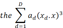
The data points that are taken as the support vectors are non-zero weights ssociated with it. To classify the outcome variable given the feature vector x, the formula in equation ten is applied. According to the equation, the ad is the “dual weight of data d, (xd.x) is the dot product of data d’s feature vector, and feature vector x”.

 

Equation 10: Due to the usage of the polynomial kernel, the dot product is raised to the power of 3

 

   

The application of the proposed approach showed that the vehicles were ultimately rejected which was the same for this procedure. The appraiser's assessment of the vehicles that had the potential to be purchased was used as the input of the SVM machine learning model. The model predicted whether the car was to be sold in less than 30 days to serve as a complement to the current procedure of decision-making.

 

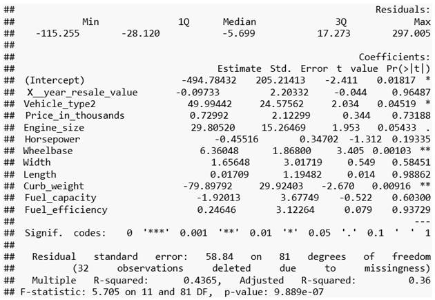
Multiple Regression Model Analysis

Steps in interpreting the multiple regression analysis start with examining the F-statistic and the associated p-value, at the bottom of the model summary.  In our example, the p-value of the F-statistic is < 9.889e-07, which is highly significant. This shows that at least, “one of the predictor variables is significantly related to the outcome variable”.  To see which predictor variables are significant, we can examine the coefficients table, “which shows the estimate of regression beta coefficients and the associated t-statistic p-values”.

Coefficients:
##                        Estimate Std. Error t value Pr(>|t|) 
## (Intercept)          -494.78432  205.21413  -2.411  0.01817 *
## X__year_resale_value   -0.09733    2.20332  -0.044  0.96487  
## Vehicle_type2          49.99442   24.57562   2.034  0.04519 *
## Price_in_thousands      0.72992    2.12299   0.344  0.73188  
## Engine_size            29.80520   15.26469   1.953  0.05433 .
## Horsepower             -0.45516    0.34702 -1.312 0.19335  
## Wheelbase               6.36048    1.86800   3.405  0.00103 **
## Width                   1.65648    3.01719   0.549  0.58451  
## Length                  0.01709    1.19482   0.014  0.98862  
## Curb_weight           -79.89792   29.92403  -2.670  0.00916 **
## Fuel_capacity          -1.92013    3.67749  -0.522  0.60300  
## Fuel_efficiency         0.24646    3.12264   0.079  0.93729  
## ---
## Signif. codes:  0 '***' 0.001 '**' 0.01 '*' 0.05 '.' 0.1 ' ' 1

       

For a given predictor, the t-statistic evaluates whether there is a significant association between the predictor and the outcome variable, that is whether the beta coefficient of the predictor is significantly different from zero. Changes in vehicle type, wheelbase, curb weight, and engine size are significantly associated with changes in sales, while changes in year's resale values, price of vehicles, horsepower, width, length, fuel capacity, and fuel efficiency are not significantly associated with car sales.  For a given predictor variable, the coefficient (β) can be interpreted as the average effect on y of a unit increase. In this predictor variable, holding all other predictors are fixed.  All the variables that are not significant, are removed from the model:  So, so the new model is computed as follows:

 

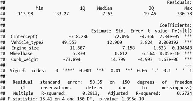
Finally, our model equation can be computed as follows: 

 

Model Accuracy Assessment

In MLR model, the R² is the “correlation coefficient between the observed values of the outcome variable (y) and the fitted (i.e., predicted) values of y”. The “value of R will always be positive and will range from zero to one.  R² represents the proportion of variance, in the outcome variable y, that may be predicted by knowing the value of the x variables”. An “R² value close to 1 indicates that the model explains a large portion of the variance in the outcome variable.  A problem with the R², is that it will always increase when more variables are added to the model, even if those variables are only weakly associated with the response James et al. (2014)”. One suggested solution will be to adjust the R² by considering the “predictor variables”.  In our data, with vehicle type, engine size, wheelbase, and curb weight, “predictor variables, the adjusted” R² = 0.2724, meaning that “27.24% of the “variance in the measure of sales can be predicted by” the variables.

 

7. Conclusion and Recommendation for Future Studies

The data mining method SVM approach implemented in this study provided just an ‘Accuracy’ of about 70% of the prediction ratio to determine whether a vehicle was sold within 30 days or less. Comparatively, the supervisor's subjective decision-making skill determines its effectiveness, and this showed over 50% of vehicles getting sold in less than 30 days or actual 30 days, while the other 50% sold in more than 30 days which may not be an adequate or desirable percentage for the company. The study showed that the four outputs in the confusion matrix to determine the performance classifier reacted positively to the objective of the study except for the ‘Accuracy’ classifier. Accuracy is an important performance matrix for data-driven decision-making based on the confusion matrix model. The practical implication of the feature selection result using the contingency table shows the assessment of 12 out of 45 aspects of a certified used vehicle should be more focused by an appraiser to generate important classification from the dataset, thereby limiting the number of criteria associated with a vehicle or car deals in terms of fulfillment and acquisition by the auto dealership.

In the multiple linear regression analysis performed to check the effect of different predictor variables on car sales, the analysis showed more explanations of dependent or explained variables as outlined and the impact of predictors on car sales. This application of the multiple regression analysis applied to data provided event to justify our model in the predictive analysis. The analysis showed only four predictor variables with a significant relationship to the car sales largely, according to this test car sales effect by vehicle type, engine size, wheelbase, and curb weight. Total variance explained by the above model showed a computation of R²= 0.2724, which means 27.24 percent of variation explained by these predictor variables. This is significant to the SVM approach implemented in this study. This represents a justification that implementing business intelligence (BI) using predictive data analytics and its machine learning models leads to “an increase in revenue, an improvement in customer satisfaction”, improved decision making, and a higher market share.

Future studies should consider different variables that may include the car's mileage, years of manufacture and/or the car's trend, or a similar number of car variants of the same brand that the company has in stock. This would help increase the model data's accuracy and help enable the data mining model approaches in determining a more functional decision-making process. The selection method performing matrix should be programmatically continuously fed using an input selection system. This makes it easier to add new features based on new trends without having an error in program utility acceptance as referenced in the contingency table.

 

8. Ethical Approval

This article does not contain any studies with human participants or animals performed by any of the authors.

 

CONFLICT OF INTERESTS

None. 

 

ACKNOWLEDGMENTS

None.

 

REFERENCES

Abidin, T. F., Rizal, S., Iqbalsyah, T. M., & Wahyudi, R. (2020). Decision Tree Classifier for University Single Rate Tuition Fee System. International Journal of Business Intelligence and Data Mining, 17(2), 258–271. https://doi.org/10.1504/IJBIDM.2020.108764

Adebiaye, R., & Conner, C. (2015). Chiropractor Practice Management: Justifications for Business Degree Program in Chiropractic Curriculum. International Journal of Advanced Scientific Research & Development (IJASRD), 02, 03(I), 01–15.

Ahadi, A. (2017). A Contingency Table Derived Method for Analyzing Course Data. Hellas, A, and Lister, R. ACM Transactions on Computing Education (TOCE), 17(3), 1–9. https://dl.acm.org/doi/abs/10.1145/3123814

Caruana, R., & Niculescu-Mizil, A. (2004). Data Mining in Metric Space: An Empirical Analysis of Supervised Learning Performance Criteria. In Proceedings of the Tenth ACM SIGKDD International Conference on Knowledge Discovery and Data Mining (pp. 69–78). https://doi.org/10.1145/1014052.1014063

Chen, C., Hao, L., & Xu, C. (2017). Comparative Analysis of Used Car Price Evaluation Models. AIP Conference Proceedings, 1839(1), 20165. https://doi.org/10.1063/1.4982530

Das, S., Mudgal, A., Dutta, A., & Geedipally, S. R. (2018). Vehicle Consumer Complaint Reports Involving Severe Incidents: Mining Large Contingency Tables. Transportation Research Record, 2672(32), 72–82. https://doi.org/10.1177/0361198118788464

Eloksari, E. A. (2020). Indonesians OPT For Secondhand Cars Amid Slowing Economy [Report], The Jakarta Post,

Flach, P. (2012). Machine learning: The Art and Science of Algorithms That Make Sense of Data. Cambridge University Press.  

Foley, É., & Guillemette, M. G. (2010). What is Business Intelligence? International Journal of Business Intelligence Research, 1(4), 1–28. https://doi.org/10.4018/jbir.2010100101

Giudici, P., & Passerone, G. (2002). Data Mining of Association Structures to Model Consumer Behavior. Computational Statistics and Data Analysis, 38(4), 533–541. https://doi.org/10.1016/S0167-9473(01)00077-9

Hočevar, B., & Jaklič, J. (2010). Assessing benefits of business intelligence systems–a case study. Management: Journal of Contemporary Management Issues, 15(1), 87–119.  

Imandoust, S. B., & Bolandraftar, M. (2013). Application of K-Nearest Neighbor (Knn) Approach for Predicting Economic Events: Theoretical background. International Journal of Engineering Research and Applications, 3(5), 605–610.

Jeffrey, A. (2018). Driving Customer Loyalty: Moving from Wished to Actions from Experian [Annual report], Experian Automotive.  

Moews, B., Herrmann, J. M., & Ibikunle, G. (2019). Lagged Correlation-Based Deep Learning for Directional Trend Change Prediction in Financial Time Series. Expert Systems with Applications, 120, 197–206. https://doi.org/10.1016/j.eswa.2018.11.027

Oprea, C. (2011). Making the Decision on Buying Second-Hand Car Market Using Data Mining Techniques. USV Annals of Economics and Public Administration, 10(3), 17–26.

Oshiro, T. M., Perez, P. S., & Baranauskas, J. A. (2012). How Many Trees in a Random Forest? BT – Machine Learning and Data Mining in Pattern Recognition (P. Perner (Ed.), Springer, 154–168.  

Peerun, S., Chummun, N. H., & Pudaruth, S. (2015). Predicting the Price of Second-Hand Cars using Artificial Neural Networks. The Second International Conference on Data Mining, Internet Computing, and Big Data (BigData2015), 17.  

Peng, C.-Y. J., Lee, K. L., & Ingersoll, G. M. (2002). An Introduction to Logistic Regression Analysis and Reporting. Journal of Educational Research, 96(1), 3–14. https://doi.org/10.1080/00220670209598786 

Pudaruth, S. (2014). Predicting the Price of Used Cars Using Machine Learning Techniques. Int. J. Inf. Computing Technology, 4(7), 753–764.  

Rish, I. (2011). An empirical study of the naive Bayes classifier. IJCAI 2001 Workshop on Empirical Methods in Artificial Intelligence, 3(22), 41–46.  

Rutkowski, L., Jaworski, M., Pietruczuk, L., & Duda, P. (2014). The CART Decision Tree for Mining Data Streams. Information Sciences, 266, 1–15. https://doi.org/10.1016/j.ins.2013.12.060

Sousanis, J. (2011). World Vehicle Population Tops 1 billion Units. Automobile Magazine, Michigan: WardsAuto. In World Vehicle Population Tops, 1 billion Units.  Science, D. (2019). Confusion Matrix. Manisha-sirsat.blogspot.com. Retrieved February 15, 2021.  

What is Business Intelligence and How It Boost Auto Dealerships? (2019). FrogData. FrogData. Retrieved February 15, 2021.  

What is Business Intelligence? Your Guide to BI and Why it Matters. (2021). Tableau. Retrieved February 15, 2021.

Zetu, D., & Miller, L. (2010). Managing Customer Loyalty in the Auto Industry. R. L. Polk&Co, 1–5