
|
|
|
|
A COMPARATIVE STUDY OF M| M | 1 AND M| M | C MODELS FOR B2C WITH SUPPLY CHAIN PROCESSGeetanjali Sharma 1 1, 2 Department of Mathematics and Statistics, Banasthali Vidyapith, Rajasthan, India |
|
|||
|
|
||||
|
Received 15 December 2021 Accepted 28 January 2022 Published 17 February 2022 Corresponding Author Geetanjali
Sharma, geetanjali.bu@gmail.com DOI 10.29121/ijetmr.v9.i2.2022.1098 Funding:
This
research received no specific grant from any funding agency in the public,
commercial, or not-for-profit sectors. Copyright:
© 2022
The Author(s). This is an open access article distributed under the terms of
the Creative Commons Attribution License, which permits unrestricted use, distribution,
and reproduction in any medium, provided the original author and source are
credited.
|
ABSTRACT |
|
||
|
With
the emerging technology of electronic commerce, most of the business
companies positively tend to offer services to their clients dealing in B2C
e-commerce. We pro- posed four models for business to consumer (B2C) with
supply chain management. First two models are M |M |1 with and without server
breakdown and other models are M |M |C with and without server
breakdown. During service when the
server breakdown, the re- pairing process of the server begins immediately.
During repair period the server serves the customer with slow rate and
service period follows exponential
distribution. Then numerical
results are also illustrated various system performances are calculated. |
|
|||
|
Keywords: M|M|1 Model, M|M|C Model, Supply Chain, B2C E-Commerce 1. INTRODUCTION Supply chain management
is an organized interrelated business network involved in the produced goods
and services required by the customers. It is a very systematic and
stratified coordination of the traditional business functions. It can be defined as
“the management of flow of products and services, which starts from the
production and ends at the consumption of products”. It also comprises moving and stored impure
materials which is involved in progressive works of inventory system and
completely furnished goods. Its target is to watch and co-relate the
production, shipment, and distribution of products and all its services. At
every step in the supply chain, it uses various ideas and approaches for its
efficient working. In this scenario companies devoted to give the best
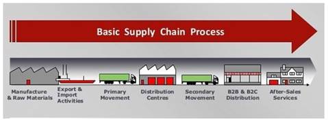
quality products to the customers and attempt to fulfill all their demands. Figure 1 shows a supply
chain management process diagram.
|
|
|||


In general, internet plays an important role to reduce the powers of third parties involved in supply chain process. Suppliers can provide offer on their products and services directly to his customers, where purchasers can also easily find what they need directly from producers like business to consumer process. This disintermediation has updated the supply chain process by facilitating the changes in demand-supply process in the market. There are some important roles that are played by internet when it comes to supply chain: Inventory management, Purchasing and transportation, Processing the orders, Relationship with vendors and Customer service etc.
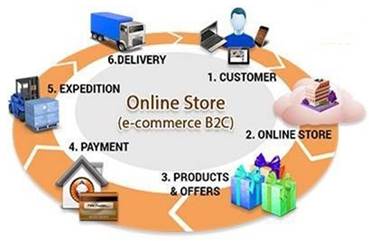
The term business-to-consumer (B2C) tends to the process of buying and selling products and services directly between the producers and consumers without involving any third party. The idea of B2C was first of all used by Mr. Michael Aldrich in 1979 by using TV as a medium for communicating with consumers. B2C is typically used to refer to on-line retailers who sell products and services to consumers by using the web services. Even now internet and its environment are a part of day-to-day life. Web applications and mobile apps behave as an interactive and important tool and with the help of them consumers, employees and others can connect to company applications using internet as a global network. Figure 2 shows a pictorial view of B2C model.
|
|
|
Figure 2 Business to Consumer Model |
Van Slyke et al. (2004) conducted a survey of consumers regarding the trust of web merchants. Also contributed the literature to the technology adoption. Sun et al. (2007) treated consumer e-commerce as a technology adoption process and discussed about the advancements of two models TAM (Technology Acceptance Model) and TTF (Task- Technology Fit Model). A theoretical framework is developed by Kim et al. (2008) for trust and risk affect an internet consumer purchasing decisions, they also test the model and implicate it. Researchers given many trust models in order to explain the factors that convince the consumers to trust e-commerce. Al-Dwairi and Kamala (2009) expanded the TAM model including necessary constructs (consumers factors, websites quality and e-vendors factors) that reflect a real acceptance of consumers for web transaction by building a trust relationship with e-vendors. Srivastava (2012) investigated a BI (Business Intelligence) system which evaluated by comparing with M |M |1 and M |D|1 queuing models. Srivastava (2013) calculated response time of various queuing models for B2C E-commerce architecture using Gang-Scheduling algorithm.
Ta et al. (2015) contributed knowledge, information, and tangible resources to supply chain management processes, consumers can co-build value for everyone, for firms and for consumers. Hence B2C collusion involves strategic leveraging of the consumer market access various activities, whereby consumers working as extra employees for firms and involved in supply chain execution without any mediator. The success of e-commerce in the era of internet, e-business model plays a key role. B2C and C2B are the mainstream model of e-business. Zhu (2015) made comparative analysis from the perspective of supply chain and e-business operation process of B2C and C2B. Yu et al. (2016) highlighted the
Logistics models and the techniques for supporting them which updated the e-commerce logistics very significantly. A model is proposed by Giannikas et al. (2017) for examining the similarities and differences between B2B and B2C warehousing which shows how the different nature of B2B and B2C commerce affects different elements of warehousing. Feng (2017) introduced a vertical B2C e-commerce network model and also discussed about its performance in two aspects: professional and specific. Bi and Liu (2018) studied the distribution centre location, transit centre location and least mile distribution strategy in the e-commerce distribution network under B2C environment. Also, a novel conceptual model is developed by Hurtado et al. (2019) for accepting the anticipation of e-commerce’s demand and to enable its predictive planning for the supply of products.
The remaining part of this paper is organized as follows: In section 2, we give the model description and the steady state solution. In section 3 we carried out a numerical study. Also calculate some system performance measures. Section 4 concludes the paper.
2. MATHEMATICAL MODEL
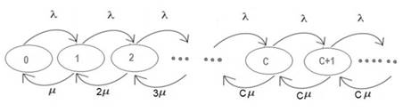
Queuing models established incredible values in many practical applications in commercial system such as production, inventory systems and supply chain management. Queuing models help us to encourage and evaluate the variability effect. In this section we con- structs four models: M |M |1 model for regular busy period, M |M |1 model with server breakdown, M |M |C model for regular busy period and M |M |C model with server break- down. Figure 3, 4, 5 and 6 respectively presents their state transition rate diagram of the proposed models.
Assumptions
1) Arrival process follows Poisson distribution and in continuously engaged period the arrival parameter is λ.
2) When the system falls in continuously engaged period it serves customers on the basis of exponential distribution with rate µ.
3) The server may break down during a service. Once the system breakdowns the effected server i.e., the server whose services are interrupted jumps to the front and repairing process to the server starts immediately. Repair period follows exponential distribution with rate α.
4) at this time (repair period) customers comes accordingly as Poisson process with rate λ1(λ1 < λ).
5) During repair period the server serves the customers, and the service follows the exponential distribution with rate µ1(µ1 < µ).
6) FIFO/(FCFS) rule is followed to selection of the customers for providing services.
2.1. M|M|1 MODEL WITH SERVER BREAKDOWN
|
|
|
Figure 3 State transition rate diagram |
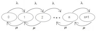
The set of balance equations are:
![]()
![]()
![]()
and
![]()
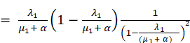
So, Equation 1 becomes
![]() Equation
2
Equation
2
Now the expected number of customers in the system and queue is:
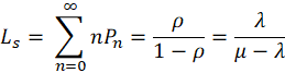
and
![]()
Expected waiting time of a customer in the system and queue, using Little’s formula:
![]()
![]()
2.2. M|M|1 MODEL WITH SERVER BREAKDOWN
|
|
|
Figure 4 State transition rate diagram |
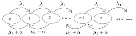
The steady state equations are:
![]()
![]()
![]()
![]()
![]()
![]()
![]()
We know that,

![]()
![]()
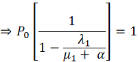
![]()
Put this value in Equation 3, we get
![]() Equation 4
Equation 4
Now expected number of customer of customers in the system and queue are:
![]()
![]()
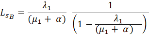
and
![]()
Average waiting time in the system and queue are:
![]()
and
![]()
2.3. M|M|C MODEL WITH REGULAR BUSY PERIOD
|
|
|
Figure 5 State transition rate diagram |
Here
![]()
![]()
So, the steady state probabilities are:
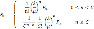
We know, Sum of all probabilities =1, Which gives
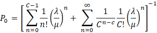
Now the expected number of customers in the queue and system is:
![]()
Employ Little’s Law L=λW. Thus, expected waiting time in the queue and system is:
![]()
![]()
![]()
![]()
![]()
2.4. M|M|C MODEL WITH BREAKDOWN
|
|
|
Figure 6 State transition rate diagram |
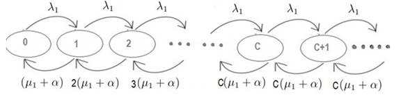
Here
![]()
![]()
So, the steady state probabilities are:
So,
![]()
Also let ![]()
Average number of customers in the queue and system are:
![]()
![]()
![]()
And
![]()
Thus, expected waiting time in the queue and system are:
![]()
and
3. NUMERICAL RESULTS
The obtained results are evaluated numerically and are based on some specific parameters. The effect of parameters in the various performance measurements are studied and also summarized in the tables given below. Table 1 shows effect of λ, Table 2 shows effect of µ, Table 3 shows effect of α, Table 4 shows effect of µ1 and Table 5 shows effect of λ1 on system performance measures. The model parameters taken in all computations are:
λ = 0.6, µ = 0.9,
λ1 = 0.4,
µ1 = 0.5, α
= 0.2 and C = 3
|
Table 1 Effect of λ |
||
|
M
|M |1 Model |
M
|M |C Model |
|
|
λ |
Ws Wq Lq |
Ws Wq Lq |
|
0.6 |
3.3333 2.2222 1.3333 |
0.5840 0.0113 0.0068 |
|
0.61 |
3.4483 2.3372 1.4257 |
0.5783 0.0118 0.0072 |
|
0.62 |
3.5714 2.4603 1.5254 |
0.5728 0.0124 0.0077 |
|
0.63 |
3.7037 2.5926 1.6333 |
0.5673 0.0129 0.0082 |
|
0.64 |
3.8462 2.7350 1.7504 |
0.5618 0.0135 0.0086 |
|
0.65 |
4.0000 2.8889 1.8778 |
0.5565 0.0141 0.0092 |
|
0.66 |
4.1667 3.0556 2.0167 |
0.5513 0.0147 0.0097 |
|
0.67 |
4.3478 3.2367 2.1686 |
0.5461 0.0153 0.0103 |
|
0.68 |
4.5455 3.4343 2.3354 |
0.5410 0.0160 0.0109 |
|
0.69 |
4.7619 3.6508 2.5190 |
0.5361
0.0166 0.0115 |
|
0.7 |
5.0000 3.8889 2.7222 |
0.5312 0.0173 0.0121 |
|
Table 2 Effect of µ |
||
|
M
|M |1 Model |
M |M |C Model |
|
|
µ |
Ws Wq Lq |
Ws Wq Lq |
|
0.9 |
3.3333 2.2222 1.3333 |
1.1266 2.2222 0.0093 |
|
0.91 |
3.2258 2.1269 1.2761 |
1.1138 2.1269 0.0089 |
|
0.92 |
3.1250 2.0380 1.2228 |
1.1012 2.0380 0.0085 |
|
0.93 |
3.0303 1.9550 1.1730 |
1.0889 1.9550 0.0082 |
|
0.94 |
2.9412 1.8773 1.1264 |
1.0769 1.8773 0.0079 |
|
0.95 |
2.8571 1.8045 1.0827 |
1.0652 1.8045 0.0075 |
|
0.96 |
2.7778 1.7361 1.0417 |
1.0537 1.7361 0.0072 |
|
0.97 |
2.7027 1.6718 1.0031 |
1.0425 1.6718 0.0069 |
|
0.98 |
2.6316 1.6112 0.9667 |
1.0315 1.6112 0.0067 |
|
0.99 |
2.5641 1.5540 0.9324 |
1.0208 1.5540 0.0064 |
|
1 |
2.5000 1.5000 0.9000 |
1.0103 1.5000 0.0062 |
|
Table 3 Effect of α |
||
|
M
|M |1 Model |
M |M |C Model |
|
|
α |
WsB LqB WqB |
WsB WqB LqB |
|
0.2 |
3.3333 1.3333 0.5333 |
2.0597 0.0597 0.0239 |
|
0.21 |
3.2258 1.2258 0.4903 |
2.0601 0.0601 0.0241 |
|
0.22 |
3.1250 1.1250 0.4500 |
2.0606 0.0606 0.0242 |
|
0.23 |
3.0303 1.0303 0.4121 |
2.0611 0.0611 0.0244 |
|
0.24 |
2.9412 0.9412 0.3765 |
2.0615 0.0615 0.0246 |
|
0.25 |
2.8571 0.8571 0.3429 |
2.0620 0.0620 0.0248 |
|
0.26 |
2.7778 0.7778 0.3111 |
2.0624 0.0624 0.0250 |
|
0.27 |
2.7027 0.7027 0.2811 |
2.0629 0.0629 0.0251 |
|
0.28 |
2.6316 0.6316 0.2526 |
2.0633 0.0633 0.0253 |
|
0.29 |
2.5641 0.5641 0.2256 |
2.0637 0.0637 0.0255 |
|
0.3 |
2.5000 0.5000 0.2000 |
2.0641 0.0641 0.0256 |
|
Table 4 Effect of µ1 |
||
|
M
|M |1 Model |
M
|M |C Model |
|
|
µ1 |
WsB WqB LqB |
WsB WqB LqB |
|
0.5 |
3.3333 1.3333 0.5333 |
2.0351 0.0351 0.0141 |
|
0.51 |
3.2258 1.2650 0.5060 |
1.9933 0.0325 0.0130 |
|
0.52 |
3.1250 1.2019 0.4808 |
1.9532 0.0302 0.0121 |
|
0.53 |
3.0303 1.1435 0.4574 |
1.9148 0.0280 0.0112 |
|
0.54 |
2.9412 1.0893 0.4357 |
1.8779 0.0261 0.0104 |
|
0.55 |
2.8571 1.0390 0.4156 |
1.8425 0.0243 0.0097 |
|
0.56 |
2.7778 0.9921 0.3968 |
1.8084 0.0227 0.0091 |
|
0.57 |
2.7027 0.9483 0.3793 |
1.7755 0.0212 0.0085 |
|
0.58 |
2.6316 0.9074 0.3630 |
1.7439 0.0198 0.0079 |
|
0.59 |
2.5641 0.8692 0.3477 |
1.7135 0.0185 0.0074 |
|
0.6 |
2.5000 0.8333 0.3333 |
1.6840 0.0174 0.0070 |
|
Table 5 Effect of λ1 |
||
|
M
|M |1 Model |
M |M |C Model |
|
|
λ1 |
WsB WqB LqB |
WsB WqB LqB |
|
0.4 |
3.3333
1.3333 0.5333 |
2.0597
0.0597 0.0239 |
|
0.41 |
3.4483
1.4483 0.5938 |
2.0645
0.0645 0.0264 |
|
0.42 |
3.5714
1.5714 0.6600 |
2.0696
0.0696 0.0292 |
|
0.43 |
3.7037
1.7037 0.7326 |
2.0750
0.0750 0.0323 |
|
0.44 |
3.8462
1.8462 0.8123 |
2.0807
0.0807 0.0355 |
|
0.45 |
4.0000
2.0000 0.9000 |
2.0867
0.0867 0.0390 |
|
0.46 |
4.1667
2.1667 0.9967 |
2.0931
0.0931 0.0428 |
|
0.47 |
4.3478
2.3478 1.1035 |
2.0998
0.0998 0.0469 |
|
0.48 |
4.5455
2.5455 1.2218 |
2.1068
0.1068 0.0513 |
|
0.49 |
4.7619
2.7619 1.3533 |
2.1142
0.1142 0.0560 |
|
0.5 |
5.0000
3.0000 1.5000 |
2.1220
0.1220 0.0610 |
4. CONCLUSION
Electronic commerce (e-commerce) means commercial process is dealt by e-media and internet. Business-to-consumer (B2C) is one of the types of electronic commerce. Orders are placed through internet, but deliveries are made at the customer’s home. In this paper, a comparative study of M|M|1 and M|M|C queuing models are discussed. Also, we calculate the performance measures and found the results for B2C with supply chain management.
REFERENCES
Al-Dwairi, R. M. and Kamala, M. A. (2009). An integrated trust model for business-to- consumer (b2c) e-commerce : Integrating trust with the technology acceptance model. En 2009 International Conference on Cyber Worlds, pages 351-356. IEEE. Retrieved from https://doi.org/10.1109/CW.2009.34
Bi, X. Q. and Liu, C. (2018). E-commerce distribution network optimization research based on b2c.
Feng, X. (2017). Research on the strategic transformation of vertical b2c e-commerce industry. En 2017 4th International Conference on Education, Management and Com- puting Technology (ICEMCT 2017). Atlantis Press. Retrieved from https://doi.org/10.2991/icemct-17.2017.227
Giannikas, V., Woodall, P., McFarlane, D., and Lu, W. (2017). The impact of b2c com- merce on traditional b2b warehousing. In 22nd International Symposium on Logistics : Data Driven Supply Chains, pages 375-383. Nottingham University Business School. Retrieved from https://www.researchgate.net/profile/Vaggelis-Giannikas/publication/321315173_The_impact_of_B2C_commerce_on_traditional_B2B_warehousing/links/5a1c20f3aca272df080f602d/The-impact-of-B2C-commerce-on-traditional-B2B-warehousing.pdf
Hurtado, P. A., Dorneles, C., and Frazzon, E. (2019). Big data application for e-commerce's logistics : A research assessment and conceptual model. IFAC- Papers OnLine, 52(13) :838-843. Retrieved from https://doi.org/10.1016/j.ifacol.2019.11.234
Kim, D. J., Ferrin, D. L., and Rao, H. R. (2008). A trust-based consumer decision-making model in electronic commerce : The role of trust, perceived risk, and their antecedents. Decision support systems, 44(2) :544-564. Retrieved from https://doi.org/10.1016/j.dss.2007.07.001
Srivastava, R. (2012). Mathematical model using bi for improving e-commerce businesses applicability's. The International Research Journal of IT and Science Management (IRJITSM). Retrieved from https://www.researchgate.net/profile/Rashad-Al-Saed/publication/312595851_Mathematical_model_using_BI_for_improving_E-Commerce_Businesses_applicability's/links/5e7df9d692851caef4a2d9fc/Mathematical-model-using-BI-for-improving-E-Commerce-Businesses-applicabilitys.pdf
Srivastava, R. (2013). Evaluation of response time using gang scheduling algorithm for b2c electronic commerce architecture implemented in cloud computing environment by queuing models. International Journal of Future Computer and Communication, 2(2) :71. Retrieved from https://doi.org/10.7763/IJFCC.2013.V2.124
Sun, J., Ke, Q., and Cheng, Y. (2007). Study of consumer acceptance in e-commerce by integrating technology acceptance model with task-technology fit model. En 2007 International Conference on Wireless Communications, Networking and Mobile Computing, pages 3621-3624. IEEE. Retrieved from https://doi.org/10.1109/WICOM.2007.895
Ta, H., Esper, T., and Hofer, A. R. (2015). Business-to-consumer (b2c) collaboration : Rethinking the role of consumers in supply chain management. Journal of business logistics, 36(1) : 133-134. Retrieved from https://doi.org/10.1111/jbl.12083
Van Slyke, C., Belanger, F., and Comunale, C. L. (2004). Factors influencing the adoption of web-based shopping : the impact of trust. ACM SIGMIS Database: The DATABASE for Advances in Information Systems, 35(2): 32-49. Retrieved from https://doi.org/10.1145/1007965.1007969
Yu, Y., Wang, X., Zhong, R., and Huang, G. Q. (2016). E-commerce logistics in supply chain management : Practice perspective. Procedia Cirp. Retrieved from https://doi.org/10.1016/j.procir.2016.08.002
Zhu, Y. (2015). The comparative analysis of c2b and b2c. International Journal of Marketing Studies, 7(5) : 157 Retrieved from https://doi.org/10.5539/ijms.v7n5p157
|
|
 This work is licensed under a: Creative Commons Attribution 4.0 International License
© IJETMR 2014-2022. All Rights Reserved.