Original Article

Structure, Segment and Grid Reliabilities: A Proposal

 

 

INTRODUCTION

Every year, climatic events such as hurricanes and ice storms cause severe damage to overhead utility lines. The main component of a post-storm system rebuilding process is the hardening of the electrical power infrastructure to prevent future damage and reduce or eliminate outages due to structural failures. This can be performed in various ways, including using only engineered pole materials to guarantee a reliable structural capacity and/or upgrading existing pole designs to achieve better structural reliability, and thereby, resilience. The significance of this effort can be assessed from the fact that about 150 million wood utility poles are in service across North America. Some studies Kalaga, S. (2013). Composite Transmission and Distribution Poles: A New Trend. Energy Central Grid Network. indicate that about 3.6 to 3.7 million wood poles are replaced each year in addition to installation of 1.9 million new poles.

A significant amount of research has been performed in the past on structural reliability Utilities One. (2023, September). Transforming Grid Infrastructure with Pole Upgrades [Brochure]. New Jersey., Kalaga, S., Jayanti, P., and Kalyanaraman, A. (2024). Wind and Ice Loads on Transmission Structures: A State-of-the-Art Review. European Journal of Theoretical and Applied Sciences, 2(6)., Kalaga, S., Holmes, S., and Fecht, G. (2023). Structural Reliability of Wood and Composite Poles Subject to Hurricane Winds. Canadian Journal of Pure and Applied Sciences, 17(3), 5775–5782.. Most studies are focused on evaluating individual structure or pole reliabilities, not the surrounding grid. 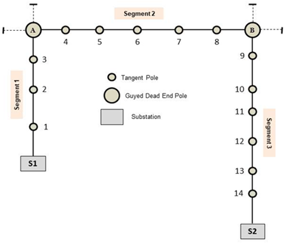To the extent the author knows, there is no specific study aimed at connecting the calculated structural or pole reliabilities to that of the line segment and then relate them to the line or overall grid itself (see Figure 1). This study is a small step in that direction and focuses on poles within a line segment between dead ends and between terminal substations. Only tangent, self-supporting poles are considered. Guyed and DDE (double dead end) poles are not considered since they are subject to minimum bending and therefore have greater nominal reliability. This article is also intended only to suggest exploring a possible means of computing grid reliability and does not purport to present a definitive solution to the problem.  

 

 

The definitions of climactic loads and their variations, and regulatory criteria, are briefly discussed in the next sections. These definitions refer to the North American subcontinent but can be adjusted to reflect local conditions at any other location.

 

BACKGROUND

Between the early 80’s to 2017, continental USA witnessed a 10-fold increase in frequency of severe climate events where nearly 80% of the outages are weather-related Kenward, A., and Raja, U. (2014). Blackout: Extreme Weather, Climate Change and Power Outages. Climate Central.. This experience led policymakers and utility stakeholders to focus on developing the necessary tools and processes that can describe and quantify reliability of the utility grid. One of the benefits of upgrading a utility grid infrastructure is improved reliability, and therefore, resilience, which are interdependent.

Resilience can be of two types: Operational and Infrastructure Panteli, M., and Dimitri, N., et al. (2017). Power Systems Resilience Assessment: Hardening and Smart Operational Enhancement Strategies. Proceedings of the IEEE, 105(7).. Operational Resilience refers to maintaining operational strength and robustness during a severe climactic event. Infrastructure Resilience refers to the physical strength of a power system for minimizing damage or preventing collapse. This explicitly implies the performance of the pole structures supporting the utility cables and equipment. The North American Electric Reliability Corporation. (2007). Definition of Adequate Level of Reliability. defines Reliability as a combination of Adequacy and Ability of a physical system to withstand unexpected disturbances without losses. From an engineering viewpoint, this refers to pole reliability.

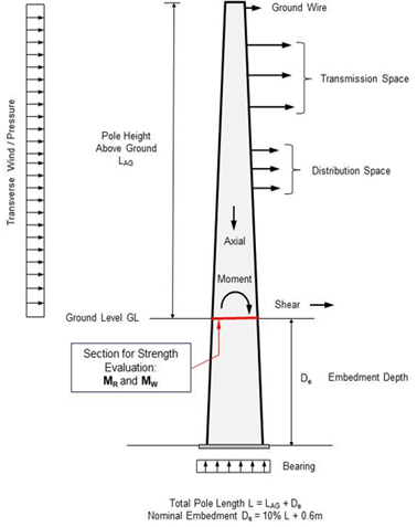
Referring to Figure 2, most tangent poles are directly embedded into the ground to a given depth. Design is governed by bending moments at the ground line and embedment depth needed to resist lateral overturning forces.

Wood, where used, is a bio-degradable material, and therefore from a structural perspective, strength reduction factors are normally specified in wood design to account for the statistical variation, decay and decrease of wood strength with time American National Standards Institute. (2017). American National Standard for Wood Poles—Specifications and Dimensions (ANSI O5-1)., Institute of Electrical and Electronics Engineers. (2023). National Electrical Safety Code (ANSI C2-23).. For others (steel, concrete, composite), no such reduction applies. A typical single-circuit transmission pole, with an overhead ground wire and under-build distribution is shown in Figure 2 but the concepts are applicable to any tangent utility pole (and poles with line angles less than 2 degrees) with a specified geometry, load points and loading regimen. 

 

GOVERNING CRITERIA

Utility structures in the United States Institute of Electrical and Electronics Engineers. (2023). National Electrical Safety Code (ANSI C2-23). and Canada Canadian Standards Association. (2015). Canadian Standards for Overhead Systems (CSA C22.3). Mississauga, Ontario, Canada., and elsewhere in the world, are designed on the basis of Load and Resistance Factor Design (LRFD) American Society of Civil Engineers. (2019). Manual of Practice no. 74: Guidelines for Electrical Transmission Line Structural Loading (4th ed.). Reston, VA. where the statistical variability of applied loads is matched with that of the resistance to reduce the potential for failure. 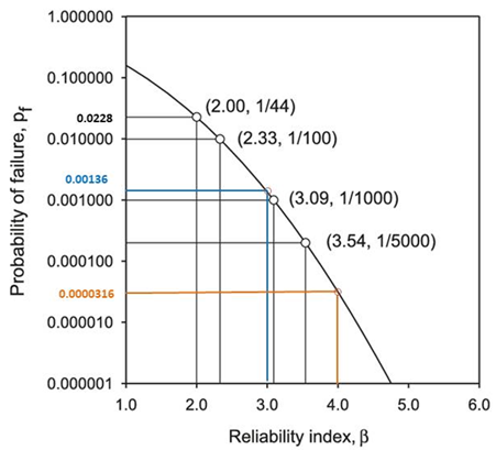This method is also called Reliability-Based Analysis and Design (RBAD) since it provides a specified level of design reliability based on the occurrence of climactic events such as hurricanes and ice storms. Figure 3 shows a typical relationship between Reliability Index β and Probability of Failure Pf. Engineers often use a target value of β = 3.0 as a reasonable design goal to achieve. The complimentary relationship between β and the Probability of Success is shown in Table 1. For any β of 2.5 and above, the chance of success approaches 1.0.

 

Table 1 Probability of Success for Selected Values of Reliability Index
Reliability Index	Probability of Success
1	0.81
1.5	0.9332
2	0.9772
2.5	0.99379
3	0.99865
3.5	0.999767
4	0.9999683
4.5	0.9999966
5	0.999999981

 

This β index is dependent on the MRI (mean recurrence interval, in years) of the climactic events. The MRI provides a time-based perspective on the likelihood of extreme events while the Reliability Index quantifies the structural safety. It can be also seen that the MRI and β are inversely related through the probability of failure. That is, a structure designed for a higher MRI will have a lower probability of failure and consequently a higher reliability index. The current ASCE standards stipulate a minimum MRI of 100 years, although the codes American Society of Civil Engineers. (2019). Manual of Practice no. 74: Guidelines for Electrical Transmission Line Structural Loading (4th ed.). Reston, VA. provide for consideration up to 300 to 700 years, should one need a much stronger long-term design safety.

For more understanding of the various loading criteria and structural element resistance related to an RBAD, the reader is referred to the abundant literature available on the topic Ang, A. H.-S., and Tang, W. H. (1984). Probability Concepts in Engineering Planning and Design. John Wiley and Sons., Kharmanda, G., and El-Hami, A. (2016). Reliability in Biomechanics (1st ed.). John Wiley and Sons., Kalaga, S., and Yenumula, P. (2017). Design of Electrical Transmission Lines: Structures and foundations (1st ed.). CRC Press.. The standards of reliable performance of utility pole structures are discussed in American Society of Civil Engineers. (2006). Manual of Practice no. 111: Reliability-Based Design of Utility Pole Structures. Reston, VA..

 

Some basic features of RBAD, as used in this study, and referring to Figure 3, are as follows.

The definition of a Reliability Index β for a normally distributed variable is:

 

                                                                                                                                   (1)

 

where:

M_R = Mean value of Resistance                                                

M_W = Mean Value of Applied Load Effect (as a function of MRI)                      

σ_R = Standard Deviation of Resistance = (COVR) (MR)

σ_W = Standard Deviation of Load Effect = (COVW) (MW)

COV_R = Coefficient of Variation of Resistance

COV_W = Coefficient of Variation of Load Effect

Load Effect MW is the applied bending moment at the ground line (GL) due to vertical and lateral loads; Resistance MR is the bending moment capacity at the ground line based on section properties. 

From statistical perspectives, pole resistance MR is a random variable, and most pole strengths are historically known to follow a Normal (Gaussian) Distribution. Loading MW on utility poles in North America, both transmission and distribution, is limited to effects of ice and wind. While the magnitude and occurrence of these loads vary with their geographical location, their effect is manifested in single poles as GLBM (ground line bending moment). Radial ice accumulation on wires is known to follow a Normal Distribution Transportation Research Board. (2003). NCHRP report 489: Design of Highway Bridges for Extreme Events. Washington, DC. but wind speeds are a different proposition. Low-to-moderate winds 64 kmph to 96 kmph (40 mph to 60 mph) are often assumed to follow a Weibull Distribution with higher winds 145 kmph (90 mph) and above taken to be an Extreme Value Type 1 (EVT) Distribution. These distributions can be 2- or 3- parameter distributions depending on the approach adopted Ellingwood, B. R., and Tekie, P. B. (1999). Wind Load Statistics for Probability-Based Structural Design. Journal of Structural Engineering, 125(4)., Simiu, E., Lombardo, F. T., and Yeo, D. H. (2012). Discussion on Ultimate Wind Load Design Gust Wind Speeds Effects in the United States for Use in ASCE 7. Journal of Structural Engineering, 138(5).. Previous studies also suggested that wind speed distributions concurrent with ice are best described by a Weibull Distribution.

The values of COV’s of loads and resistances vary widely depending on location, topography and MRI of climactic loads. For example, some typical values often cited in the industry are:

Wood COVR = 0.17 to 0.20 applied to the bending stress American National Standards Institute. (2017). American National Standard for Wood Poles—Specifications and Dimensions (ANSI O5-1).

Steel, Concrete and Composite Poles COVR = 0.05 (nominal)

COV_W = 0.08 to 0.10 applied to the wind load (general) Joffre, S. M., and Laurila, T. (1988). Standard Deviations of Wind Speed and Direction from Observations Over a Smooth Surface. Journal of Applied Meteorology, 27(5).

                 = 0.13 (EVT-1 Distribution, 100-year MRI) Ellingwood, B. R., and Tekie, P. B. (1999). Wind Load Statistics for Probability-Based Structural Design. Journal of Structural Engineering, 125(4). 

COV_W = 0.18 applied to the radial ice Transportation Research Board. (2003). NCHRP report 489: Design of Highway Bridges for Extreme Events. Washington, DC.

Equation 1 cannot be used in situations where one of the variables is non-normal. In such cases, the evaluation must consider any of the alternative theoretical methods such as variate transformation to Normal Distribution, Box-Cox transformation, Monte Carlo Simulation (MCS) etc. The accuracy of the transformations depends on the values of the location, scale and shape parameters of the parent EV distributions, especially those of high wind speeds Bureau of Indian Standards. (1995). Institute of Standards and Technology. (2015). Maps of Non-Hurricane and Non-Tornadic Wind Speeds with Specified MRIs for the Contiguous United States Using a Two-Dimensional Poisson Process Extreme Value Model and Local Regression (NIST Special Publication 500-301)..

 

Separation of Ice and Wind Reliability Components

Alternatively, if the situation involves both normal (ice) and non-normal (wind) variables, then the pole reliability can be considered as a sum of individual reliabilities β_n and β_nn (for example, when the load effect involves both ice and wind). That is, the load effects are considered and processed separately.

 

                                                (2)

 

In the event that the governing loading is just wind (non-normal), Equation 2 reduces to:

 

                                                                                                               (3)

 

In the event that the governing loading is just ice (normal), Equation 2 reduces to:

 

                                                                                                                        (4)

 

PROPOSED   MODEL

We propose a simple model for grid reliability index as applied to a hypothetical North American grid shown in Figure 1. The grid runs between 2 substations S1 and S2 and contains 3 segments: S1 to A, A to B and B to S2. The segments taken together constitute a line or grid with 14 tangent poles with different effective spans. Poles A and B are dead ends and rarely fail as they are guyed in both directions. The load cases shown in Table 2 give typical weather loading for this model.

It must be noted that this is NOT a comprehensive, global model but only offers guidance towards developing such models for other locations. Weather is most South Asian countries such as India is mostly dominated by high winds and high temperatures Bureau of Indian Standards. (1995). IS 802-1-1: Structural Steel in OHTL Towers: Part 1—Loads, Materials and Permissible Stresses. New Delhi, India. and the model can be appropriately adjusted to such situations. The model implicitly assumes that statistical data related to the main variables is readily available. For example, in the continental USA, climactic wind and ice data is collected and processed by National Institute of Standards and Technology. (2004). Extreme Wind Speeds: Overview (NIST Publication 898). Washington, DC, United States. with the help of hundreds of weather stations located strategically across the country.   

 

Assumptions

1)       Each pole’s structural reliability index is an explicit function of the pole’s strength under a given set of controlling load cases as applied to the spans comprising the segment.

2)       Statistical variation of applied load effects and pole resistances is known and data is available. 

3)       Poles considered for the process are tangent poles (zero to small line angles, <= 2o)

 

 

Table 2 Typical Weather and Load Cases
LC No.	Description	Radial Ice Thickness (mm)	Wind Speed  (kmph)	Wind	Comment	Assumed Distribution
				Load
				(kPa)
LC1	District Load Case	0	96	431	Light	Ice: Normal Wind: Weibull
		6	64	192	Medium
		12	64	192	Heavy
LC2	Extreme Wind	0	145 to 241	991 to 2758	Location- dependent	Extreme Value Type 1
LC3	Combined Ice and Wind	12 to 25	Variable	Variable	Location- dependent	Ice: Normal Wind: Weibull
LC4	Heavy Ice on Conductors	25 to 75	0	0	Location- dependent	Ice: Normal
*non-standard, but utility-mandated load based on local experience   **See IEEE-Institute of Electrical and Electronics Engineers. (2023). National Electrical Safety Code (ANSI C2-23). for various values based on location (1 inch = 25.4 mm, 1 psf = 47.88 kPa, 1 mph = 1.608 kph)

 

Individual Pole Reliability Index βi

Each pole reliability index βi is the lowest of those computed for the 4 load cases shown in Table 2. Note that loading cases LC1 and LC3 contain both ice and wind and this implies presence of two different random variates with different distributions. As mentioned before, the analytical treatment of the situation requires either a variate transformation to Normal or a Monte Carlo Simulation with specified COVs, plus consideration of Equation 2 (or 3, as required).

 

                              β_i = Minimum (β_iLC1, β_iLC2, β_iLC3, β_iLC4); i = 1 to 14                                                                                                    (5)

 

If we assume that Extreme Wind (LC2) controls the design of tangent poles at that location, then Equation 5 can be reduced to:

 

                                        β_i = Minimum (β_iLC2); i = 1 to 14                                                                                                                     (6)

 

If we assume that Extreme Ice (LC4) controls the design of tangent poles at that location, then Equation 5 can be reduced to:

 

                                                  β_i = Minimum (β_iLC4); i = 1 to 14₎                                                                                                             (7)

 

Segments

This idealization assumes that effects of any structural failure in a segment will be confined to that segment. The pole system in each segment is analogous to a connected set of components (poles) where failure of any one unit leads to the failure of the entire segment. Additionally, the reliability of the segment is a function of the lowest component (pole) reliability, often called the “weakest link” of the system. When the failure of each component is independent of the others, the reliability of the segment, β𝑠eg is the taken equal to the lowest reliability of the individual components.

 

                                                  β_𝑠eg = Min [β₁, β₂, β₃ … β_𝑛]                                                                                                                     (8)

 

β𝑛 is the reliability of the nth component (pole) in the segment.  

For the entire grid of Figure 1we define Segment Reliabilities simply as follows:

 

                                                  β_seg1 = Min [β₁, β₂, β₃]                                                                                                 (9a)

 

                                                      β_seg2 = Min [β₄, β₅, β₆, β₇, β₈]                                                                                            (9b)

 

                                                β_seg3 = Min [β₉, β₁₀, β₁₁, β₁₂, β₁₃, β₁₄]                                                                                  (9c)

 

Grid Reliability can now be simply defined as an RMS average of the 3 segment minimums:

 

                                             βG = √ [(β2seg1 + β2seg2 + β2seg3)/3]                                                                              (10)

 

Knowledge of individual βis and grid βGs can help utility planners identify weak spots within the grid and take remedial action before the next catastrophic climactic event. Poles with lesser β values can be either replaced or upgraded to enhance the overall segment and grid.

 

APPLICATION

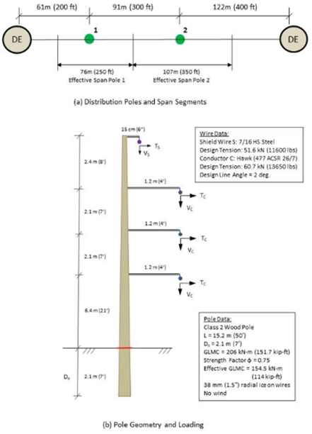
To illustrate the computational concepts discussed above, a small 2-pole, 3-span segment between dead ends (see Figure 4a) is considered. The load case considered is Extreme Ice (LC4 of Table 2) with radial ice thickness of 38 mm (1.5 inches), normally distributed. The structure loading for the single circuit pole (Figure 4b) consisted of vertical loads Vs and Vc and transverse loads Ts and Tc (due to line angle) applied at the end of davit arms. Values of the loads Ts and Tc corresponding to a line angle of 2 degrees are calculated using Excel spreadsheets and standard equations from textbooks Kalaga, S., and Yenumula, P. (2017). Design of Electrical Transmission Lines: Structures and foundations (1st ed.). CRC Press.. 

The following numerical values are used in the calculations:

M_W1 = 96.5 kN-m (71.2 kip-ft)

M_R1 = MR2 = 154.5 kN-m (114 kip-ft)(identical poles)

M_W2 = `104.2 kN-m (76.8 kip-ft)

COV_W = 0.18 (ice)

COV_R = 0.20 (wood)

σ_R1 = σ_R2 = (COV_R)  (M_R) = 0.20  154.5 = 30.9 kN-m (41.9 kip-ft)

σ_W1 = (COV_W)  (M_W1) = 0.18  96.5 = 17.4 kN-m (12.8 kip-ft)

σ_W2 = (COV_W)  (M_W2) = 0.18  104.2 = 18.8 kN-m (13.9 kip-ft)

From Equations 1 and 4, the reliability indices for the poles are:

β_pole1 = 1.64   β_pole2 = 1.39  Minimum of β_pole1 and β_pole2: 1.39

Therefore, Segment Reliability R = 1.39

The value of Probability of Success is about 0.906.

If the segment were to use steel poles of the same height and capacity instead of wood, the reliability increases several-fold as shown below:

M_W1 = 96.5 kN-m (71.2 kip-ft)

M_R1 = M_R2 = 206 kN-m (151.7 kip-ft) (no strength reduction)

M_W2 = `104.2 kN-m (76.8 kip-ft)

COV_W = 0.18 (ice)

COV_R = 0.05 (steel)

 σ_R1 = σ_R2 = (COV_R)  (M_R) = 0.05  206 = 10.3 kN-m (7.6 kip-ft)

σ_W1 = (COV_W)  (M_W1) = 0.18  96.5 = 17.4 kN-m (12.8 kip-ft)

σ_W2 = (COV_W)  (M_W2) = 0.18  104.2 = 18.8 kN-m (13.9 kip-ft)

 

From Equations 1 and 4, the reliability indices for the poles are:

β_pole1 = 5.41   β_pole2 = 4.75  Minimum of βpole1 and βpole2: 4.75            

Therefore, Segment Reliability R = 4.75

The value of Probability of Success is about 0.999999.

 

This example has only one segment; in the event there are more, Equations 9 and 10 come into play.

Selecting steel as a pole material will provide for a higher pole/segment reliability owing to the low coefficient of variation associated with steel strength. In the above example, steel pole minimum reliability is about 3.4 times that of wood for the specific load case considered. A similar level of reliability is also observed for composite poles Kalaga, S., Holmes, S., and Fecht, G. (2023). Structural Reliability of Wood and Composite Poles Subject to Hurricane Winds. Canadian Journal of Pure and Applied Sciences, 17(3), 5775–5782., Kalaga, S., Jayanti, P., and Kalyanaraman, A. (2024). Wind and Ice Loads on Transmission Structures: A State-of-the-Art Review. European Journal of Theoretical and Applied Sciences, 2(6)..

 

CONCLUSIONS

In the previous sections, we discussed the definitions of reliability and resilience and proposed a simple mathematical model for the structural reliability of a small grid. Ground line resistance of a tangent pole is considered along with load effects resulting from wind and ice. Mathematical expressions are proposed to connect the individual pole reliabilities to segment values and then to the overall line. An important inference from this brief study is that explicit, location-dependent statistical distributions of the climactic variables are essential to accurately evaluate individual pole reliabilities. The computations are somewhat simplified if high wind loading controls the behavior of a tangent pole and Equation 3 can be employed.

The application of the concepts is illustrated with a 3-span, 2-pole segment containing wood and steel poles subject to Extreme Ice loading. 

The next step of this continuing study is finding a way to numerically evaluate Equations 1, 2, 3 and 4 and then the subsequent expressions 5 to 9. Efforts are presently directed towards that goal. The suggestion to separate the “effects” of the variables (say, wind and ice) per Equation 2, and define βi accordingly, should be investigated further. Computing the structural reliability index of each pole first as a function of each load effect separately and then assessing its minimum value seems to be a rational approach. Reasonably good grid reliability estimates can assist in identifying weak spots and in maintaining reliable transmission and distribution lines.

This study considered only poles, but the theoretical basis can be applied to other structural systems including concrete, laminated wood and composite poles.

 

REFERENCES

American National Standards Institute. (2017). American National Standard for Wood Poles—Specifications and Dimensions (ANSI O5-1).

American Society of Civil Engineers. (2006). Manual of Practice no. 111: Reliability-Based Design of Utility Pole Structures. Reston, VA.

American Society of Civil Engineers. (2019). Manual of Practice no. 74: Guidelines for Electrical Transmission Line Structural Loading (4th ed.). Reston, VA.

Ang, A. H.-S., and Tang, W. H. (1984). Probability Concepts in Engineering Planning and Design. John Wiley and Sons.

Bureau of Indian Standards. (1995). IS 802-1-1: Structural Steel in OHTL Towers: Part 1—Loads, Materials and Permissible Stresses. New Delhi, India.

Canadian Standards Association. (2015). Canadian Standards for Overhead Systems (CSA C22.3). Mississauga, Ontario, Canada.

Ellingwood, B. R., and Tekie, P. B. (1999). Wind Load Statistics for Probability-Based Structural Design. Journal of Structural Engineering, 125(4). https://doi.org/10.1061/(ASCE)0733-9445(1999)125:4(453)

Haynes, R. (2011). How to Transform a Weibull Distribution. Smarter Solutions.

Institute of Electrical and Electronics Engineers. (2023). National Electrical Safety Code (ANSI C2-23).

Joffre, S. M., and Laurila, T. (1988). Standard Deviations of Wind Speed and Direction from Observations Over a Smooth Surface. Journal of Applied Meteorology, 27(5). https://doi.org/10.1175/1520-0450(1988)027

Kalaga, S. (2013). Composite Transmission and Distribution Poles: A New Trend. Energy Central Grid Network.

Kalaga, S., and Yenumula, P. (2017). Design of Electrical Transmission Lines: Structures and foundations (1st ed.). CRC Press. https://doi.org/10.1201/9781315755687    

Kalaga, S., Holmes, S., and Fecht, G. (2023). Structural Reliability of Wood and Composite Poles Subject to Hurricane Winds. Canadian Journal of Pure and Applied Sciences, 17(3), 5775–5782.

Kalaga, S., Holmes, S., and Fecht, G. (2024). Reliability of Distribution Poles: Supply-Demand Perspectives. In CIGRE Canada Conference, Winnipeg, Manitoba, Canada.

Kalaga, S., Holmes, S., and Fecht, G. (2024, May). Reliability of Wood and Composite Distribution Poles. In IEEE PES TandD Conference, Anaheim, CA, United States. https://doi.org/10.1109/TD47997.2024.10556232

Kalaga, S., Jayanti, P., and Kalyanaraman, A. (2024). Wind and Ice Loads on Transmission Structures: A State-of-the-Art Review. European Journal of Theoretical and Applied Sciences, 2(6). https://doi.org/10.59324/ejtas.2024.2(6).56

Kenward, A., and Raja, U. (2014). Blackout: Extreme Weather, Climate Change and Power Outages. Climate Central.

Kharmanda, G., and El-Hami, A. (2016). Reliability in Biomechanics (1st ed.). John Wiley and Sons. https://doi.org/10.1002/9781119370840

National Institute of Standards and Technology. (2004). Extreme Wind Speeds: Overview (NIST Publication 898). Washington, DC, United States.

Bureau of Indian Standards. (1995). Institute of Standards and Technology. (2015). Maps of Non-Hurricane and Non-Tornadic Wind Speeds with Specified MRIs for the Contiguous United States Using a Two-Dimensional Poisson Process Extreme Value Model and Local Regression (NIST Special Publication 500-301).

North American Electric Reliability Corporation. (2007). Definition of Adequate Level of Reliability.

Panteli, M., and Dimitri, N., et al. (2017). Power Systems Resilience Assessment: Hardening and Smart Operational Enhancement Strategies. Proceedings of the IEEE, 105(7). https://doi.org/10.1109/JPROC.2017.2691357

Simiu, E., Lombardo, F. T., and Yeo, D. H. (2012). Discussion on Ultimate Wind Load Design Gust Wind Speeds Effects in the United States for Use in ASCE 7. Journal of Structural Engineering, 138(5). https://doi.org/10.1061/(ASCE)ST.1943-541X.0000341

Transportation Research Board. (2003). NCHRP report 489: Design of Highway Bridges for Extreme Events. Washington, DC.

Utilities One. (2023, September). Transforming Grid Infrastructure with Pole Upgrades [Brochure]. New Jersey.