NEURO-FUZZY INTELLIGENT CONTROLLER FOR LFC OF A FOUR-AREA POWER SYSTEM

 

Basavarajappa Sokke Rameshappa ¹ , Nagaraj Mudakapla Shadaksharappa ¹

 

¹ Department of Electrical and Electronics Engineering, Bapuji Institute of Engineering and Technology, Davanagere, VTU, Belagavi, India

 

1. INTRODUCTION

An automatic load frequency control is essential to maintain system stability in complex power system operations. It is possible by controlling the system frequency and the power flows in tie-lines, which are at nominal values for small perturbations in demand Kundur (1994). An automatic LFC in the power system reduces the area control error (ACE). ACE is the summation of the tie-line power and system frequency deviation. The speed changer position of the governor is adjusted using a servo-motor mechanism in the secondary loop of the control area. The drawbacks of conventional PID controllers are – slow response and high undershoot/overshot in the ACE. Artificial Intelligent (AI) controllers can overcome these drawbacks. 

In Shaker et al. (2019), an adaptive LFC for a single area using ANFIS and an artificial intelligence technique is employed. The genetic algorithm is used to tune the PID controller. A three-area interconnected power system with fuzzy logic self-tuned PID controller is employed for LFC problems. A hybrid neuro-fuzzy-based ANFIS controller and robust fuzzy logic-based fine-tuning approach are proposed for frequency control in a three-area hydrothermal system Khezri et al. (2016). An ANFIS approach is proposed for LFC in a multi-area power generation system, and its performance is compared with conventional controllers Prakash and Sinha (2017). A distributed model predictive LFC for a four-area hydrothermal power system is proposed. The controller is designed based on optimal control theory  Zhang et al. (2017). A multi-source power system's automatic LFC with the ANFIS approach is presented considering GRCs and other non-linearity Bhaskar et al. (2018).

The research work in the literature employs hybrid techniques combining conventional and artificial intelligent controllers without GRC to minimize the ACE. It also employs predictive model control and ANFIS approach with GRC but does not provide several epochs, optimization techniques, and dynamics of steam turbines. Hence, the present research proposes an ANFIS controller that uses ACE and the derivative of ACE to train the model for the LFC system with steam turbine dynamics, GRC, hybrid, and backpropagation optimization techniques.

 

2. MATERIALS AND METHODS

2.1. DEVELOPMENT OF THE POWER SYSTEM MODEL

The dynamic mathematical models of various components of power plants were presented in IEEE: Power and Energy Society. (2013). For thermal plants, a governor's transfer function (TF) model is derived from the fundamental speed governor operation as given in Equation 1.

 

                                                                                         Equation 1

 

The TF models of a single reheat, tandem compound steam turbine, are obtained from the turbine dynamics as given in Equation 2, Equation 3, Equation 4, for the turbine, reheater, and crossover.     

      

                                                                                                      Equation 2

                                                                                           Equation 3

                                                                                                      Equation 4

 

For a nuclear plant, the TF model of a speed governor is derived as given in   Equation 5.

                                                                                                    Equation 5

The TF models of a double reheat tandem compound steam turbine are obtained from the turbine dynamics as given in Equation 6, Equation 7, Equation 8, for the turbine, reheater, and crossover, respectively.

 

                                                                                          Equation 6

                                                                                          Equation 7

                                                                                          Equation 8

 

For a hydropower plant, the TF model of a hydro governor is derived as given in Equation 9.

 

                                                           Equation 9

 

The TF model of a hydro turbine [3] is obtained from the turbine dynamics, as given in Equation 10.

 

                                                                                             Equation 10

 

where             = hydro governor reset or washout time constant. = hydro governor temporary droop.

The presence of GRC in the system affects stability Sahin (2020). The GRCs for all areas are included by adding the limiters to the turbines. The alternator and load TF model is obtained from the Swing equation as given in Equation 11. 

 

                                                                     Equation 11

 

where = mechanical power,  = electrical power, and  = acceleration power.

Equation 11 can be written in the standard form is obtained as given in  Equation 12.

 

   , for i = 1, 2, 3, 4.                                            Equation 12

 

In the system operation, the power flow on the tie-lines is given in Equation 13.

 

                                                                           Equation 13

 

The deviation in tie-line power flow is derived from the power angle equation as  Equation 14

 

                                                     Equation 14

 

ACE is the error signal fed to the controller and is derived as, the combination of the change in tie-line power and system frequency, given in Equation 15.

 

                           for i, j = 1, 2, 3, 4.                              Equation 15

 

The integral of time-weighted absolute error (ITAE) is considered an objective function and is calculated as given in Equation 16.

 

   for i, j = 1, 2, 3, 4.                                  Equation 16

 

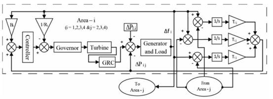
Figure 1 shows the connection of the various components of i^th area in a four-area multi-source power system. This system comprises a hydro, a nuclear, and two thermal power plants.

Figure 1

                                                                      

Figure 1 Power System Model

 

2.2.  CONVENTIONAL PID CONTROLLER

Ziegler and Nichols have suggested a method to calculate the controller gain values. The values of critical gain  and the critical period   are used for calculation of the gain values, as shown in Table 1, using the gain equations given below: 

 

                                                                                           Equation 17

                                                                                            Equation 18

.                                                                               Equation 19

 

 

 

 

 

Table 1

Table 1 PID Controller Parameters
Plant
Thermal	0.286	12.289	0.177	0.028	0.264
Nuclear	0.181	19.137	0.109	0.012	0.261
Hydro	0.112	16.885	0.067	0.008	0.142

 

2.3. SUGENO FUZZY LOGIC CONTROLLER

Takagi-Sugeno-Kang proposed an approach for developing fuzzy rules from the given input-output data. Sugeno fuzzy inference system (a knowledge or rule-based) is used in this non-linear power systems with uncertainty. In this controller, the inputs are fuzzifying and then applying the fuzzy operator, but membership functions in the output are either constant or linear. A rule in the Sugeno model consists of two inputs, error (p) and derivative of error (q), and an output (r). This rule is given by

IF p is X and q is Y, THEN r is r = f (p, q)

where X and Y are the linguistic variables, and f (p, q) is a polynomial function of p and q.

The inference system is a zero-order model if f (p, q) is a constant and is a first-order model if f (p, q) is a linear function of p and q. Because each rule has a crisp output, the overall output is obtained via the weighted average defuzzification method. The defuzzification is done through the weighted average method. Table 2 shows the fuzzy associative memory (FAM) table to form forty-nine rules with triangular membership functions, and the output function is taken as a constant to obtain the fuzzy inference system (fis) file.

Table 2

Table 2 FAM Table
Rule Bases		Derivative Error (DACE)
		NB	NM	NS	Z	PS	PM	PB
Error	NB	PB	PB	PM	PM	PS	PS	Z
(ACE)	NM	PB	PM	PM	PM	PS	Z	Z
	NS	PB	PM	PM	PM	Z	NS	NS
	Z	PB	PM	PM	Z	NS	NM	NB
	PS	PM	PM	NS	NS	NM	NB	NB
	PM	PM	PS	NS	NM	NB	NM	NB
	PB	NS	NS	NM	NM	NM	NM	NB

 

2.4.  ANFIS CONTROLLER

It combines neural network and fuzzy logic algorithms to obtain a Sugeno-type fis file. It is designed using a hybrid learning rule with backpropagation. The gradient descent optimization method is used to obtain the training data. The two rules and five layers of the ANFIS structure are shown in Figure 2.

 

R1: IF x is & y is ,  THEN

R2: IF x is & y is , THEN

 

where , and , are the linguistic variables. , , and, ,are the consequent parameters.

The training data set is collected from Sugeno fuzzy logic controller outputs. This data is uploaded in the anfis editor to generate the fis file. The grid partitioning technique with 5x5 gbell and linear type membership functions are used. The generated fis file is used in training the data set with hybrid and backpropagation optimization techniques for 20 epochs. The process of training and testing the data is repeated until the error reduces to . Generate the fis file with the gbell function for all four areas separately. This file is used in the ANFIS controller to simulate the power system and get the desired output.

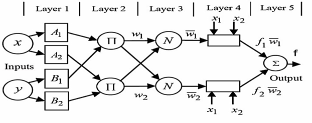Figure 2

Figure 2 ANFIS Architecture

 

3. RESULTS AND DISCUSSIONS

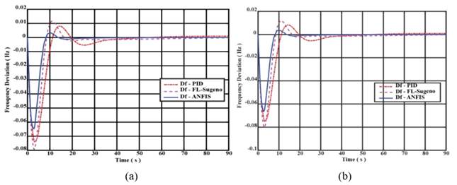
The system parameters are given in Appendix A at a nominal frequency  of 50 Hz. The simulation of a developed power system model is performed for each type of controller. The simulation is carried out using Matlab. Consider the case with a 1% step load increase simultaneously in all the areas (A1 to A4); the frequency deviation  with three types of controllers is shown in Figure 3 and Figure 4. As the load increases, the speed decreases, and hence frequency decreases.

Further, the speed increases due to the primary control action by the speed governor and the secondary control action by the ANFIS controller. This results in zero ACE deviation. It is evident from the simulation results that the proposed controller reduced the steady state error and improved the transient responses in terms of undershoot, settling time, and the smaller value of ITAE.

Figure 3

                                                       

Figure 3  With 1% Load Increase in (a) A1 and (b) A2

Figure 4

                                                             

Figure 4  with 1% Load Increase in (a) A3 and (b) A4

 

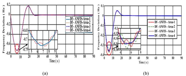
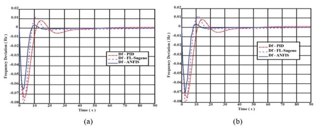
The step change in load  from 1% to 4% in each area is considered. The ITAE values and the step response characteristics, undershoot , and settling time , are measured in each case. Table 3 shows the comparative study of characteristics and error values for each case. Figure 5 (a) shows the  with ANFIS controller under 4% step load change (equal load). The transient specifications are the settling time of 27.9823 sec (min) and undershoot of - 0.7374 Hz (min) with an ITAE value of 1.541, which are measured. These specifications are acceptable and smaller compared to conventional controllers. Figure 5 (b) shows the  with ANFIS controller under  in each area. Its dynamic response is good with a very minimum steady.

Table 3

Table 3 Settling Time, Maximum Undershoot and ITAE of Frequency Deviation
Load	Controllers	Settling Time (sec)				Maximum Undershoot (Hz)				ITAE
		A1	A2	A3	A4	A1	A2	A3	A4
+1 %	PID	37.4276	37.0483	37.4279	36.7415	-0.0741	-0.0752	-0.0741	-0.0749	0.1128
	Fuzzy	35.3831	24.1459	35.3825	23.7027	-0.0793	-0.0802	-0.0793	-0.0798	0.0903
	ANFIS	12.5448	12.6491	12.5449	12.2472	-0.0647	-0.0664	-0.0647	-0.0692	0.0255
+2 %	PID	31.4877	31.4790	31.4883	31.3404	-0.2334	-0.2341	-0.2334	-0.2358	0.3229
	Fuzzy	18.4069	18.3627	18.4069	18.3300	-0.2346	-0.2352	-0.2346	-0.2378	0.2314
	ANFIS	16.2255	16.2110	16.2255	15.8983	-0.2289	0.2289	0.2289	-0.2333	0.3635
+3 %	PID	25.8549	25.7815	25.8546	25.8021	-0.4649	-0.4649	-0.4649	-0.4714	0.8842
	Fuzzy	21.8765	21.8081	21.8767	21.7396	-0.4647	-0.4648	-0.4647	-0.4713	0.7378
	ANFIS	20.8092	20.6850	20.8092	20.7816	-0.4606	-0.4606	-0.4606	-0.4682	0.8374
+4 %	PID	48.2282	48.7783	48.2355	47.6003	-0.7440	-0.7440	-0.7440	-0.7503	1.9070
	Fuzzy	39.8828	57.6070	39.8753	39.8705	-0.7424	-0.7424	-0.7424	-0.7497	2.0750
	ANFIS	28.0254	29.2096	27.9823	28.9171	-0.7374	-0.7374	-0.7374	-0.7426	1.5410

 

Figure 5

                                                                     

Figure 5  with ANFIS Controller Under (a) Equal Load and (b) Unequal Load

 

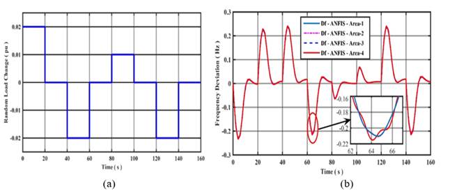
The robustness of the ANFIS controller with a random load curve, as shown in Figure 6 (a), is assessed for all four areas, and the frequency deviations ( are shown in Figure 6 (b). It is observed that the ANFIS controller exactly tracks the load curve as the load increases the system frequency decreases. It matches the generation with load demand and losses at a constant frequency. For the case with an equal change in load, frequency deviation occurs in the respective areas which are less than the threshold value.

For the system with the proposed ANFIS controller, the values of  and  at a 3% change in load, these values are - 0.4606 Hz (min) and 20.6850 sec (min), respectively. For a 2% change in load, these values are - 0.2289 Hz (min) and 15.8983 sec (min), respectively, and at a 1% change in load, these values are further reduced to - 0.0647 Hz (min) and 12.2472 sec (min), respectively. Thus, the obtained time response characteristics are smaller compared to the values given in the literature by Deepesh Sharma (2020) and Feng Liu (2017). Hence, the proposed ANFIS controller is more effectively tuned with GRCs than PID and FL controllers.

Figure 6

                                                                     

Figure 6 (a) Random Load Curve and (b)  with ANFIS Controller Under Random Load

 

4. CONCLUSIONS

This research article is presented to assess the effectiveness of an ANFIS controller in four control areas with different sources connected through tie-lines. Transient analysis is carried out, considering the tandem compound TF models of steam turbines and the nonlinearity of GRC under equal and unequal loads. The Z-N method is employed to tune the controller gains and minimize the value of ITAE. The simulation of the model for an equal change in load shows that the proposed ANFIS controller provides a very significant improvement. Its dynamic step responses have smaller values of specifications compared to conventional and fuzzy logic controllers. The proposed controller is robust and quickly adaptable to nonlinearity in the system. Also, this work shows that the ANFIS controller performs very effectively even under random demand changes, and thus the power system stability is achieved.

 

5. NOMENCLATURE

: Power system rated capacity, : Nominal load, : Tie-line power, : Load damping constant, : Frequency bias factor, : Inertia constant, : Governor speed regulation,    : Nominal frequency,  : Frequency deviation, : Power angle, : Synchronizing torque co-efficient, : Power system gain, : Power system, Governor, Turbine, Reheater, Crossover time constants, respectively, , ,, : Fraction of turbine power at HP, LP, IP and VHP sections respectively, : Turbine water starting time constant, : Hydro governor reset time constant, : Hydro governor temporary droop, : Hydro governor permanent droop.

 

6. SYSTEM PARAMETERS

= 2000MW, = 1000MW, = 200MW,  = 2.5Hz/pu MW,   = 30deg., = 0.0866.

For thermal plant:  = 0.01pu MW/Hz,  = 0.41pu MW/Hz,  = 5MJ/MVA, = 0.2sec,

= 0.3sec, = 7sec, = 0.4sec, = 0.3, = 0.4, = 0.3, = 100Hz/pu MW,

= 20sec. GRC =

For nuclear plant:  = 0.01pu MW/Hz,  = 0.41pu MW/Hz,  = 5MJ/MVA, = 0.2sec,

= 0.3sec, = 7sec, = 0.4sec, = 0.22, = 0.56, = 0.22, = 100Hz/pu MW, = 20sec.

For hydro plant:  = 0.015pu MW/Hz,  = 0.415pu MW/Hz,  = 4MJ/MVA, = 10sec,

= 1sec, = 5sec, = 0.2875Hz/pu MW, = 0.05Hz/pu MW, = 66.6667Hz/pu MW,

= 10.6667s. GRC =  and .

 

CONFLICT OF INTERESTS

None. 

 

 

ACKNOWLEDGMENTS

The authors are grateful to the Principal of Bapuji Institute of Engineering and Technology, Davanagere, Karnataka, for their support, encouragement, and facilities in carrying out this research.

 

REFERENCES

Bhaskar,M. K., Pal, N.S.  and Yadav, V. K. (2018). A Comparative Performance Analysis of Automatic Generation Control of Multi-Area Power System Using PID, Fuzzy And ANFIS Controllers, IEEE International Conference on Power Electronics, Intelligent Control, and Energy Systems, Delhi, India, 132-137, 2018. https://doi.org/10.1109/ICPEICES.2018.8897477.

Chandrakala, K.R.M.V. and Balamurugan.S. (2018). Adaptive Neuro-Fuzzy Scheduled Load Frequency Controller for Multi-Source Multi Area System Interconnected Via Parallel AC-DC Links, International Journal on Electrical Engineering and Informatics, 10(3), 479-490. https://doi.org/10.15676/ijeei.2018.10.3.5.

IEEE : Power and Energy Society. (2013). Technical Report on Dynamic Models for Turbine-Governors in Power System Studies, Power System Dynamic Performance Committee, PES-TR1.

Khezri, R., Golshannavaz, S., Shokoohi, S. and Bevrani, H. (2016). Fuzzy Logic Based Fine-Tuning Approach for Robust Load Frequency Control in a Multi-Area Power System, Electric Power Components and Systems, Taylor and Francis Group, 44(18), 2073–2083. https://doi.org/10.1080/15325008.2016.1210265.

Liu, F., Wang, H., Shi, Q., Wang, H., Zhang, M. and Zhao, H. (2017). Comparison of an ANFIS and Fuzzy PID Control Model for Performance in a Two-Axis Inertial Stabilized Platform, IEEE Access, 5, 12951-12962. https://doi.org/10.1109/ACCESS.2017.2723541.

Kundur. P. (1994). Power System Stability and Control, Vol. 2, New York, McGraw-Hill.

Prakash, S. and Sinha, S. K. (2017). Automatic Load Frequency Control of Six Areas Hybrid Multi-Generation Power Systems using Neuro-Fuzzy Intelligent Controller, IETE Journal of Research, 64(4), 471-481. https://doi.org/10.1080/03772063.2017.1361869.

Sahin, E. (2020). Design of an Optimized Fractional High Order Differential Feedback Controller for Load Frequency Control of a Multi-Area Multi-Source Power System with Nonlinearity, IEEE Access, 8, 12327-12342. https://doi.org/10.1109/ACCESS.2020.2966261.

Shaker, H. K., Zoghby, H.E., Bahgat, M. E. and Abdel-Ghany, A. M.(2019). Advanced Control Techniques for an Interconnected Multi Area Power System for Load Frequency Control, International Conf. on Middle East Power Systems, Tanta University, Egypt, 710-715. https://doi.org/10.1109/MEPCON47431.2019.9008158.

Sharma, D. (2020). Automatic Generation Control of Multi-Source Interconnected Power System using Adaptive Neuro-Fuzzy Inference System, International Journal of Engineering, Science and Technology, 12(3), 66-80. https://doi.org/10.4314/ijest.v12i3.7.

Sharma, D., Pandey, K., Kushwaha ,V. and Sehrawat, S. (2016). Load Frequency Control of Four-Area Hydro-Thermal Interconnected Power System through ANFIS Based Hybrid Neuro-Fuzzy Approach, International Innovative Applications of Computational Intelligence on Power, Energy and Controls with their Impact on Humanity, 144-149. https://doi.org/10.1109/CIPECH.2016.7918755.

Zhang,Y., Liu, X. and  Qu, B. (2017). Distributed Model Predictive Load Frequency Control of Multi-Area Power System with DFIGs, IEEE/CAA Journal of Automatica Sinica, 4(1), 125-135. https://doi.org/10.1109/JAS.2017.7510346.